DRAFT
Department of Mathematics, Computer Science, and Statistics
St. Lawrence University
Canton, NY 13625
Preface
I have been teaching the Introduction to Computer Programming course at St. Lawrence University since 2003. This course at St. Lawrence is the first course in the Computer Science major sequence and also satisfies a general education requirement called Quantitative and Logical Reasoning. As such, it assumes no prior programming experience, and students from across campus in a variety of disciplines take this course. These notes reflect the topics and content I have been teaching the past several years and are meant to be a companion for my lectures. For the time being these notes do not necessarily hold together as a standalone resource for learning programming in Python, though that is my ultimate goal. These notes are by no means complete with regards to the Python programming language. The examples and topics covered are only a small subset of what could be covered. I have chosen them because they are fun, engaging, and relevant to a liberal arts education and are drawn from a variety of disciplines including art, biology, physics, mathematics, and of course, computer science.
If you happen upon these notes outside of my course and you find them useful I would appreciate hearing about it.
Goals of the course include:
-
Appreciate the complexity of the software systems we encounter every day.
-
Emphasize problem solving in a precise and logical framework (the Python programming language).
-
Explore a multitude of topics in computer science such as; graphics and animation, image processing, simulation and randomness, cryptography, network communications, and much more.
1. Introduction
Computer Science is about the theory and practice of processing digital information. What is digital information? It is just numbers, bits, ones and zeros, properly arranged. Computer Science encompasses such diverse areas as networking, cryptography, security, web development, artificial intelligence, databases, computer graphics, mobile computing, audio and video processing, … a list that could continue for some time. What this has enabled is astonishing; self driving cars, social media, voice and image recognition, digital music and video streaming (e.g., Spotify and Netflix), on-line shopping and banking, digital maps and GPS. Biologists use software to analyze DNA, Doctors use software to understand how genes impact disease. Pharmacologists search for new drugs using software. Computer programming and software is the thread that knits all of these seemingly disparate areas together. It is an obvious jumping off point for introducing computer science.
A computer program (i.e., software) is developed and written in a programming language. There are, literally, thousands of programming languages, mostly dead now, but there are many hundreds still in active use.[1] About a dozen languages dominate the modern software development landscape, and many more are actively used in niche areas such as engineering and the visual arts.
The Javascript programming language (not to be confused with the Java programming language) is part of every web browser and just about every web site makes use of Javascript in some way. It might be the most heavily used programming language in the world. Most computer games are written in C or C++. Native iPhone apps are written in Objective-C or Swift, while native Android apps use Google’s version of Java or Kotlin. Statisticians and data scientists frequently use R. Scientists and engineers are partial towards MATLAB or Mathematica. Processing is a special purpose language for the visual arts. Verilog and VHDL are well established languages for designing electronic circuits. Another list that could go on. The TIOBE Index attempts to measure programming language popularity.
| A programming language is precise notation used for describing computations to be carried out by a computing device (e.g., a computer, smartphone, tablet, etc.). Like a natural language such as English or German, a programming language has an alphabet, words, grammar (syntax), and meaning (semantics). |
1.1. Software is taking over
Think about each of the following, what has changed, and if there is software behind that change.
-
How often do you go into a bank and interact with a teller? What do you use instead?
-
What has happened to book stores, from your local book store to large chain stores such as Barnes and Noble and Borders?
-
When was the last time you used a travel agent to purchase an airline ticket?
-
What has happened to DVD stores such as Blockbuster? What has taken its place?
-
What is disrupting the hotel and taxi industry?
-
What has happened to music stores where we used to purchase albums and CDs?
-
When was the last time you took a roll of film to get developed?
-
When was the last time you wrote a letter and mailed it using the post office?
-
Your smart phone is a powerful computing device, how often do you look at in a day, and what do you use it for?
-
Thinking a little further in to the future what could happen to the millions of people who drive a vehicle for a living, from taxi drivers to truck drivers?
So why study computer science? Software impacts almost all aspects of our life, it might be good to learn something about it. Marc Andreesen developed Mosaic, one of the original web browsers, wrote a now somewhat dated but important article in the Wall Street Journal, Why Software Is Eating the World.
1.2. Hello World
Python is a popular programming language used widely in industry and academia. It is used for everything from web programming, scientific computing, data science, to developing games. It is a powerful general purpose programming language and is often used in introductory programming courses because it is relatively easy to learn and get started with. So lets get started.
It is almost obligatory that Hello World be the first program one writes in any programming language. Here is our first Python program:
1
print("Hello, World!")
That is it, just the one line. And it does as you might expect, it prints the message Hello, World! on the console. But there is a lot going on in that one line, so lets break it down.
The console is a text window where Python sends the output of print statements and where the user can also enter data from input statements.
|
The built-in function print prints, to the console, the values between the parentheses. In this case the value being printed is the string literal "Hello World". A string literal in Python is a sequence of characters between double quotes or single quotes. More on string literals later.
| In programming, a string literal is also called a string constant. |
The print function can take multiple values separated by commas.
1
print("The value of pi squared is", 3.14159 * 3.14159)
produces the output
The value of pi squared is 9.869587728099999And we can see right here that 1) * is part of Python, 2) that a value is on each side of the * (syntax), and 3) that * must mean multiplication (semantics).
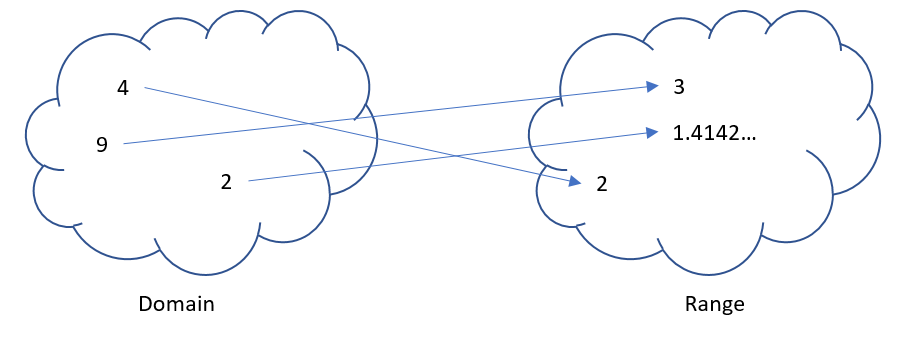
| In mathematics a function maps values in a domain to values in a range. For example, the function \(f(x) = x^2\) maps the input 2 to the output 4, 3 to 9, 1.5 to 2.25, etc. |
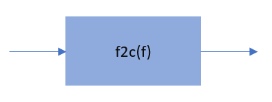
Pictorially we can think of a function as a black box (we may not know how it works) where values come in (represented by the arrow coming in on the left) and the function produces values (the return results represented by the arrow coming out of the box on the right).
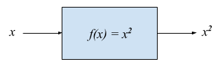
Values that are passed to a function are called arguments. The second argument in the call to the print function above is the mathematical expression 3.14159 * 3.14159. In just about every programming language the asterisk character * represents multiplication. A value such as 3.14159 in mathematics is called a real number (a number with a decimal point). For reasons I wont go into now, in computer science and programming we call real numbers floating-point numbers, or floats for short.
There is a big difference between the string literal "3.0" and the floating-point literal 3.0.
1
print("3.0 * 3.0", 3.0 * 3.0)
3.0 * 3.0 9.0Numbers without decimal points are called integers or ints for short.
1.3. Integer and floating-point literals
Valid integer literals include numbers such as 0, 1, 2, … and also negative integers -1, -2, -3, …
Don’t start an integer literal with a leading 0, such as 09. This is an error in Python.
|
Floating-point literals include a decimal place, and include numbers such as 0.3, -0.3, .3, 3., -3.14159.
Python (as do most programming languages) supports specifying numbers using scientific notation. For example, in Chemistry and Physics, Avagadro’s number is \(6.022140857 \times 10^{23}\). Writing this out as 602214085700000000000000 is not very readable. In Python we can instead write Avagadro’s number as 6.022140857e23.
| Typically if we use scientific notation we write the number so that there is one non-zero digit to the left of the decimal point. In this case we say that the number is normalized. |
We can also use scientific notation for very small numbers. The mass of an electron is \(9.10938356 \times 10^{-31}\) kg. Again, writing this as 0.000000000000000000000000000000910938356 is not helpful. We should instead write 9.10938356e-31.
| We will often also use the term constant instead of literal. An integer literal is also called an integer constant. A floating-point literal is also called a floating-point constant. A string literal is also called a string constant. |
The radius of an electron is 0.00000000000000281792 meters. Express this number using Python’s scientific notation.
2.81792e-15 # meters
1.4. Variables
Let’s return to our simple program …
1
print("The value of pi squared is", 3.14159 * 3.14159)
It would be convenient to give the value 3.14159 a name. An obvious choice being pi. We do that in Python by defining a variable using an assignment statement.
1
pi = 3.14159
And we can rewrite our program as
1
2
pi = 3.14159
print("The value of pi squared is", pi * pi)
To the left of the = sign is a variable name and we read the assignment statement above as pi gets the value of the value on the right of =, in this case 3.14159.
Variable names in Python should be meaningful. We could have said
1
2
rumpelstiltskin = 3.14159
print("The value of pi squared is", rumpelstiltskin * rumpelstiltskin)
but this makes the code less understandable.
Variable names must start with either an alphabetic character (a - z, A - Z) or underscore, and may also contain digits. Variable names are also case sensitive, so pi, Pi, and PI are all different variable names.[2]
The value on the right of = can also be an expression.
Students often confuse = with mathematical equality and think 3.14159 = pi is the same thing as pi = 3.14159. The former is not valid Python.
|
1
2
3
pi = 3.14159
pi_squared = pi * pi
print("The value of pi squared is", pi_squared)
| Variables must be defined before they are used. |
The Python program
print(x)would produce an error because the variable x does not have a value.
| Variable names are not string literals. |
1
2
print("The value of pi squared is", pi_squared) (1)
print("The value of pi squared is", "pi_squared") (2)
| 1 | prints The value of pi squared is 9.869587728099999 |
| 2 | prints The value of pi squared is pi_squaredAlmost certainly not what was intended. |
1.5. Comments
We can add notes to our program using a comment. In Python a one line comment starts with a hashtag and continues to the end of the line.
1
2
# define a variable pi
pi = 3.14159
You can also use a comment to finish a line.
1
pi = 3.14159 # define a variable named pi
1.6. Mathematical Expressions
The arithmetic operators we will be using most are:
| Operator | operation |
|---|---|
|
addition |
|
subtraction |
|
multiplication |
|
floating-point division |
|
integer division |
|
remainder (modulus) |
|
exponentiation |
Python has many more operators than shown in this table, but this is all we will need for now. You can combine these operations in complicated ways including using parentheses. The normal order of operations you learned in grade school apply.
-
parentheses
-
exponentiation
-
multiplication, division (include remainder)
-
addition and subtraction
If there are two operators at the same precedence then they should be evaluated from left to right.
For example 4 - 5 + 3 should be evaluated as (4 - 5) + 3 (which is 2) and not 4 - (5 + 3)
(which is -4).
1.6.1. Examples
What is the output of each of the examples below?
1
2
x = 3 + 5 * 9
print(x)
48
1
2
x = 1/2 (1)
print(x)
0.5
| 1 | Recall that the single slash / is floating-point division, meaning the result is
a floating-point number. |
Contrast this with integer division using the double slash operator //.
In integer division the result is always an integer.
1
2
3
4
5
w = 1 // 2
x = 3 // 7
y = 3 // 2
z = 77 // 5
print(w,x,y,z)
0 0 1 15
As we will see, integer division plays an important role in many applications in computer science.
1
2
3
4
x = 7
y = 9
z = x + y // 4 * x - 2 ** 3
print(z)
13
Expressions produce a value. Something must be done with that value such as assign it to a variable or use it as an argument in a function call (such as print). Consider the following Python program.
1
2
3
two_pi = 3.14159 * 2 (1)
two_pi * two_pi (2)
print(two_pi) (3)
| 1 | compute 2π and store the result in the variable two_pi |
| 2 | multiply two_pi times two_pi and do nothing with the result so Python just throws the value away. This line is pointless, it has no effect, but it is legal. |
| 3 | print two_pi |
1.7. Modular Arithmetic
Modular arithmetic is important in computer science. Modular arithmetic is just arithmetic that uses the remainder after finding a quotient. For example, 7 // 3 is 2 with a remainder of 1. The remainder operator is %. In this case 7 % 3 is 1.
1
2
3
4
5
6
# What gets printed by the following?
w = 1 % 2
x = 3 % 7
y = 3 % 2
z = 77 % 5
print(w,x,y,z)
1 3 1 2
A couple of important properties to remember. If we are computing n % m and we know that n is less than m and they are both positive, then the result is always n. For example 278 % 455 is 278.
In mathematics we sometimes refer to modular arithmetic as clock arithmetic. You perform modular arithmetic all the time, you just don’t know it. For example, if it is 2PM and we wanted to figure out what time it will be 14 hours from now, we can compute (2 + 14) % 12, which is 4. So it would be 4AM.
|
Computing the modulus of a negative number is also important, for example -1 % 12. Think of computing the modulus of a negative number as going counter clockwise around the clock. For example, -1 % 12 is 11, and -5 % 12 is 7.
-14 % 12 would be to go counter clockwise one full revolution leaving s with -2 % 12, which is 10.
1
2
3
4
5
6
# What gets printed by the following?
w = -1 % 2
x = -3 % 7
y = -3 % 2
z = -77 % 5
print(w,x,y,z)
1 4 1 3
| We will see a use of computing the modulus of a negative number in cryptography. |
1.8. More on String Literals
Strings are an important part of programming. Strings often seem boring but they are part of every piece of software and are often central to applications such web searching, texting, email, DNA sequence analysis, and cryptography.
A string literal is a sequence of characters between double quotes.
"This is a valid string literal"Or single quotes.
'and so is this'| The opening and closing quotes in a string literal must match. |
"but this string literal has an error, why?''and so does this, why?"But what if we want to include a single quote as one of the characters in our string literal? One way to do it is to use double quotes for the string literal.
"This isn't an error"This works because the outer double quotes demarcate the string literal and the single quote in don't is just a single quote character because it is inside the double quotes.
The following is incorrect.
'It isn't easy to see that this is an error, why?'Python can’t tell that the second single quote in isn't is part of the word but recognizes it as the closing quote matching the open quote.
1
print('He said "Do it!"')
He said "Do it!"
Things can get pretty crazy. How about if we wanted to print the string He said "Don’t do it!". The issue here is that the string we are printing contains a mix of double and single quotes. The trick is that we need to escape one of the quote characters. For example, if we need a single quote to be the single quote character and not the start or end of a string literal we can put a backslash character in front of it.
The statement
1
print('He said "don\'t do it!"')
produces the output
He said "don't do it!"1.9. A note about spaces
Spaces, like in writing, are used to separate words in Python and are often used to make code more legible. For example, in a print statement you can put a space after the comma that is separating values to print.
1
print(a, b, c, d)
which might look slightly less cramped than
1
print(a,b,c,d)
Spaces can also make code less readable,
1
print(a , b,c, d)
is also valid — but ugly.
| Spacing at the start of a line that changes indentation can cause problems. See the next section. |
1.10. A note about indentation
We will see later that indentation plays an important role in Python. For now just be aware that all Python statements that are at the same level (and we wont really know what that means until we get to more complicated Python) should be indented exactly the same.
Here is an example. The following program is in error because the second statement is indented one space.
1
2
x = 4
print(x*x)
| Python is unique in the way that it treats indentation and spacing. Most other programming languages are not sensitive to the way that indentation is handled and programmers are free to indent as they see fit to make their programs more legible. Not so in Python. Indentation is part of the syntax of the language. |
1.11. Syntax Errors
We’ve already encountered ways in which we can violate the rules of the language. In computer programming we call these syntax errors.
| A syntax error is an error that violates the rules of of how you put together the tokens (words) of the language. Syntax errors can be detected before the program executes. |
Find the syntax error in each of the following:
print("Hello)
Missing double quote closing the string literal "Hello".
print("Hello')
Mismatched quotes.
print("Hello"
Missing closing parentheses.
print("Hello" 77)
Missing comma between Hello and 77.
print(x)
Variable x is not defined.
 x = 5
print(x)
Indentation error
x = 5 9
print(x)
Python expects there to be something between the 5 and the 9 such as a mathematical operator + or *. Unless the programmer meant the integer 59
in which case there should be no space at all.
5 = x
print(x)
Python expects there to be a variable to the left of =, not an expression.
x = 8 @ 7
print(x)
Python does not have an operator named @.
Some syntax errors are just nasty and difficult to find. The following one line program looks like it should have a syntax error. It is nonsensical but shows a common mistake of leaving off the parentheses when calling a function. But the program actually runs.
<built-in function print>
As you gain practice you will be able to quickly find syntax errors.
| A built-in function is a function that is predefined by Python and is part of the Python programming language. |
1.12. Keyboard Input
Python’s input function allows the user to enter input from the keyboard. It takes a string as an argument and uses it as a prompt to display on the Python console. The input function is a different kind of function than the print function. The print function puts values on the Python console window whereas the input function produces a string value of the characters that the user typed.
1
2
name = input('Enter your name: ')
print("Hello", name)
Enter your name: Hermione (1)
Hello Hermione
| 1 | Hermione is what the user typed and then hit enter on the keyboard. |
It is common to have users enter numbers and then use the values in mathematical expressions. The formula to convert a temperature in Fahrenheit to Celsius is \(5/9(f-32)\)
1
2
3
f = input('Enter a temperature (F): ')
c = 5/9*(f - 32)
print(f, "Fahrenheit is", c, "Celsius")
Unfortunately f contains a string, not a number, and (f - 32) has an error because you can’t subtract 32 from a string. For example, if the user typed 75 it would be like trying to
compute "75" - 32, which is as bad as trying to compute "hello" - 32. You need to first convert the value in the variable f to either
an integer or a floating-point number using either the int or float function.
The input function returns a string value, even if the user entered a number. You must convert the string to a number using the int or float function if you intend to use the input in a mathematical expression.
|
int functionThe function int takes a string argument and attempts to convert it to an integer and return the resulting integer. For example int("-36") would return the integer -36. The int function is also used to convert a floating-point number to an integer by truncating the decimal point. For example int(3.14159) would return 3. Sometimes int can result in a run-time error. For example int("3.14159") causes an error because the string cannot converted to an integer. What about int('hello')?
| A run-time error is an error that can only be detected when the program executes and not before. A run-time error is often called a crash. You’ll often hear programmers say "The program is crashing" or "the program crashes on this line of code". |
|
The
The function float functionfloat takes a string argument and attempts to convert it to a floating-point number and return the resulting float. For example int("-3.14") would return the float -3.14. The float function is also used to convert an integer to a float. For example float(3) is 3.0. Similar to int if the argument cannot be converted then a run-time error will result. For example float('hello').
|
Here is our modified program:
1
2
3
f = float(input('Enter a temperature (F): ')) (1)
c = 5/9*(f - 32)
print(f, "degrees Fahrenheit is", c, "degrees Celsius")
| 1 | Notice the use of the function float to convert the string in f to a floating-point number. |
Here is a sample run of the Fahrenheit to Celsius conversion program.
Enter a temperature (F): 83.5 (1)
83.5 degrees Fahrenheit is 28.61111111111111 degrees Celsius
| 1 | The user entered 83.5 |
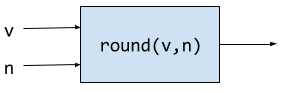
The result 28.61111111111111 has an unhelpful number of digits. It looks ridiculous. Python has a built-in function round that rounds a floating-point number to a certain number of decimal places. For example, round(3.157, 2) will round 3.157 to two decimal places, producing the value 3.16. Using this in our temperature conversion program:
1
2
3
f = float(input('Enter a temperature (F): '))
c = 5/9*(f - 32)
print(f, "degrees Fahrenheit is", round(c,1), "degrees Celsius") (1)
| 1 | Use round to round the value in`c` to one decimal place. |
Here is a sample run of the Fahrenheit to Celsius conversion program.
Enter a temperature (F): 83.5
83.5 degrees Fahrenheit is 28.6 degrees Celsius
There are two different kinds of functions in Python, those that return values, and those that do not return a value but perform some other side effect. print is an example of a function that does not return a value but has the the side effect of printing a value on the console window. Contrast this to the round function which returns a rounded result.
|
1.12.1. Program Flow
Python programs execute line-by-line top-to-bottom. Variables must be defined and assigned values before those values can be used. Consider the previous Celsius-to-Fahrenheit conversion program.
The first assignment statement that executes defines the variable f.
f = float(input('Enter a temperature (F): '))
The second statement execute defines c by using the variable f
c = 5/9*(f - 32)
Finally, the third statement executed prints the result using both c and f.
print(f, "degrees Fahrenheit is", round(c,1), "degrees Celsius")
1.13. The math module
Python has many support libraries that we can use. Think of
a support library as predefined functions and definitions that you can use. One such support library is called the math module. The math module contains many math related functions and some predefined constants. For example math.sin(x) computes the sin of the argument \(x\) (where \(x\) is in radians).
| A module is a named collection of related functions and definitions. Modules can be hierarchical, that is we can have modules defined inside other modules. Much like on your computer where you can have folders inside folders to organize your documents. |
To use the functions and definitions in the math module your program first needs to tell Python that we need it using an import statement.
1
import math
One way to compute the square root of a number would be just to raise to the 1/2 power.
print(2**.5)Another way would be to use the math module’s square root function.
1
print(math.sqrt(2))
import is a Python keyword. A keyword is a word reserved for use by Python.
As such you should never use a keyword as a variable name (in fact that is an error).
|
A constant defined in the math module is math.pi
1
print(math.pi)
3.141592653589793
To reference functions and definitions in a module use dot notation. For example, math.pi or math.sqrt(x).
|
1.13.1. Function Composition
A powerful programming technique is to call a function and use its return result as an argument in another function call. This is called function composition. Mathematically if \(f\) and \(g\) are functions that return a result we can compose them as \(f(g(x))\).
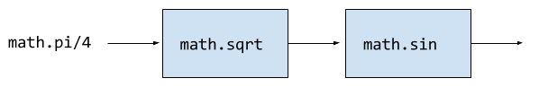
For example, if we needed to compute \(sin(\sqrt{\pi/4})\) …
1
2
result = math.sin(math.sqrt(math.pi/4)) (1)
print(round(result, 2)) (2)
| 1 | This is the function composition of math.sin and math.sqrt. |
| 2 | Here we are composing print and round |
We could have done all this in one (albeit less readable) line …
1
print(round(math.sin(math.sqrt(math.pi/4)), 2))
Or we could have also broken it up into more statements …
1
2
3
4
result1 = math.sqrt(math.pi/4)
result2 = math.sin(result1)
result3 = round(result2, 2)
print(result3)
These are all equivalent and one is not necessarily better than the other. A fourth version reuses the result variable in each statement and does not define new variables.
1
2
3
4
result = math.sqrt(math.pi/4)
result = math.sin(result)
result = round(result, 2)
print(result)
We will see over and over that there are many ways to express the same computation, some may be better than others because they are more readable or more efficient.
1.14. Kinds of Program Errors
We have already discussed syntax errors and run-time errors.
Recall that a syntax error is an error in how you put together the words and characters of your program. For example, a missing parentheses, or quote in a string literal. Syntax errors can be detected before you run the program and are often highlighted in whatever IDE [3] you are using.
A run-time error is an error that cannot be detected before program execution but only while the program is executing. Common run-time errors include dividing by zero or trying to convert the word hello to an integer. For example, consider the following simple program:
1
2
s = int(input("Enter a number: "))
print("1000 divided by", s, "is", 1000/s)
What would happen if the user entered a 0 at the input prompt? There is no way for Python to know what the user is going to type, and if they enter a 0, then the program will crash on line 2. If the user enters the word "hello" then the program will crash on line 1 when Python tries to convert "hello" to an integer.
1.14.1. Logic Errors
There are even more insidious and difficult to find errors. At least with a syntax error the IDE will tell you where in the code the error is, and when you have a run-time error Python will tell you exactly which line caused the crash.
Lets revisit our Celsius to Fahrenheit conversion program. The program below does not contain a syntax error nor does it contain a run-time error. There is, however, a problem with it. Can you see it?
1
2
3
f = float(input('Enter a temperature (F): '))
c = 5/9 * f-32
print(f, "degrees Fahrenheit is", round(c,1), "degrees Celsius")
There are parentheses missing around the f-32. This program executes just fine and produces a result, it is just the wrong result. This kind of error is a logic error. A logic error is an error where the program produces an incorrect result when it executes.
1.15. Bits, CPUs, Interpreters, and Compilers
At its most basic level everything about modern computing boils down to, at some base level, ones and zeros, true/false, on/off, yes/no, black/white. All information is binary. All decimal (base-10) numbers are expressed in binary (base-2). Digital images are just numbers, which are binary. Digital music on Spotify or Pandora, are numbers (hence binary) that represent sampled sound waves. Characters, letters, punctuation, all have a numeric equivalent, and are binary. Internet communication - binary, web pages - binary. Even computer programs get converted to binary. All information is binary.
An individual 1 or 0 is called a bit, for binary digit. Eight bits are a byte. We often talk of sizes of data in bytes. A megabyte (MB) is one million bytes. Strictly speaking when we use the term megabyte it usually means \(2^{20}\) bytes rather then \(10^6\) bytes. Below is a table of sizes, kilobytes, megabytes, …
kilobyte (KB) |
\(10^{3} = 1000\) (one thousand) |
\(2^{10}\) |
megabyte (MB) |
\(10^{6} = 1,000,000\) (one million) |
\(2^{20}\) |
gigabyte (GB) |
\(10^{9}\) (one billion) |
\(2^{30}\) |
terabyte (TB) |
\(10^{12}\) (one trillion) |
\(2^{40}\) |
petabyte (PB) |
\(10^{15}\) (one quadrillion) |
\(2^{50}\) |
exabyte (EB) |
\(10^{18}\) (one quintillion) |
\(2^{60}\) |
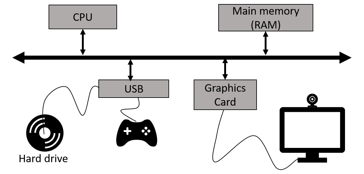
The CPU, (Central Processing Unit) or processor, carries out basic mathematical operations such as addition and multiplication. The CPU is connected to main memory where it can store numbers (bits). Main memory is fast and volatile. That is, when the power is turned off main memory loses any information that was stored. Also connected to the CPU and memory are other hardware components such as hard drives, graphics card, and network hardware. Hard drives are non-volatile memory. Turn off the power and they remember what was stored, they are also much slower than main memory.
Here is a high level layout of a computer.
The basic operations of the CPU are called instructions, and the binary representation of instructions is called machine code. Many programming languages are compiled languages that are translated to machine code by a compiler, C being the most common compiled language, where the program is converted straight to machine code that is then directly executed by the CPU.
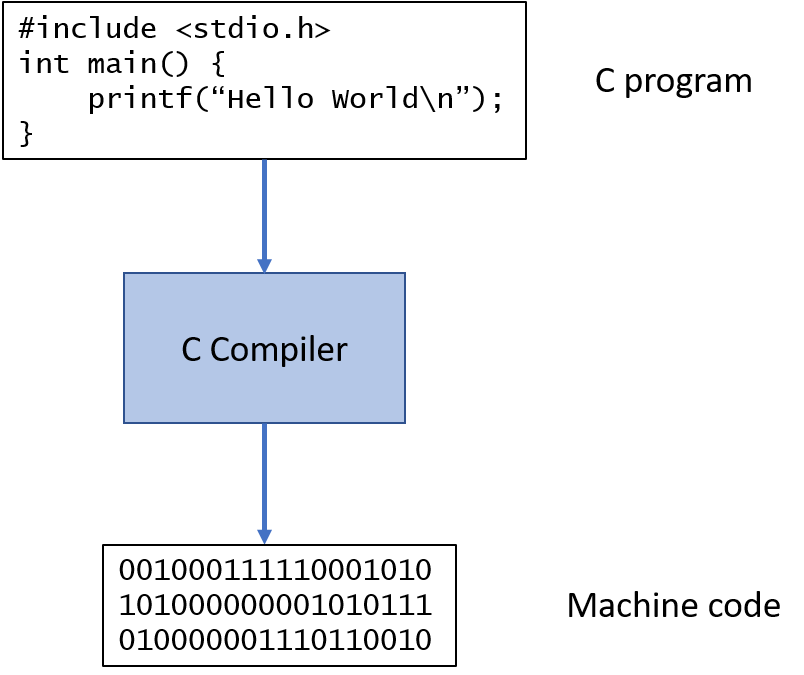
Python is a little different, it is not a compiled language but an interpreted language. What that means is that there is another program called the interpreter that reads the Python program and executes it directly. The Python interpreter itself is written in C.
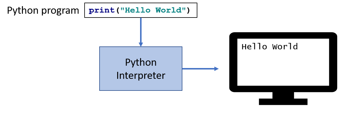
| Python is actually a bit more complicated. The Python interpreter actually compiles Python programs to a CPU independent intermediate language called byte code. It is the Python program’s byte code that is then executed the Python interpreter. |
1.16. Exercises
x and y are variables that have been assigned values. What does the following code fragment do? (Hint: give sample values to x and y and follow the code).t = x
x = y
y = tIt switches the values of x and y using the intermediate variable t.
For example, if x contained the value 3 and y contained the value 4 then after the code executed x would be 4 and y would be 3.
1
2
x = 2.0
y = math.sqrt(x)
math is a (a) function (b) module (c) variable (d) literal
(b) math is a module.
sqrt is a (a) function (b) module (c) variable (d) literal
(a) sqrt is a function.
The line x = 2.0 is an example of a/an (a) variable (b) floating-point literal (c) function call (d) assignment statement
(d) assignment statement, because x is assigned the value 2.0.
The line math.sqrt(x) in the second line is an example of (a) function composition (b) a function call (c) an argument (d) a module call
(b) function call. In choice (d), the term module call is nonsense.
In the line y = math.sqrt(x), x is an example of a (a) variable (b) module (c) argument (d) floating-point literal
This is a little tricky. If we had to choose only one answer, choice (a) variable is correct, but choice (c) argument is more precise, so it is a better answer.
1
2
3
4
z = 3
x = 2
y = z ** x // x * z
print(y)
12
The output of print(27 % 12) is?
3
The output of print(-12 % 10) is?
8
The value 0.00023 can be written as a normalized number in Python’s scientific notation as …
2.3e-4
1.17. Programming Exercises
Write a program that converts a temperature in Celsius to Fahrenheit. Prompt the user for the temperature and print the conversion rounded to two decimal places. Make the output neat and descriptive.
Write a Python program that calculates the wind chill temperature \(W\) given the current temperature \(t\) (in Fahrenheit) and the wind velocity \(v\) (in MPH). The current temperature and the wind velocity should be entered by the user from the keyboard.
The formula the National Weather Service uses to calculate wind chill temperature is:
\(W = 35.74 + 0.6215t + (0.4275t - 35.75)v^{0.16}\)
Enter temperature (F): 32.0
Enter wind velocity (MPH): 10.0
The wind chill for 32.0 degrees with a
wind velocity of 10.0 MPH is 23.7 degrees.
Print the result rounded to one decimal place, like the 23.7 above.
The area of a circle with radius \(r\) is \(area = \pi r^2\). Write a program that prompts the user for a radius and computes and prints the area of the circle rounded to 3 decimal places.
The volume of a cone with height \(h\) and radius \(r\) is \(v = \pi r^2h/3\). Write a Python program that will read the radius and the height from the user and computes and prints the volume of the cone.
In the United States there is a birth every 8 seconds, a death every 12 seconds, and a new immigrant (net) every 33 seconds. The current population is roughly 325 million. Write a program that will prompt the user for a number of years and print the estimated population that many years from now.
Assume that \(C\) is an initial amount of an investment, \(r\) is the yearly rate of interest (e.g., \(.02\) is \(2\%\)), \(t\) is the number of years until maturation, \(n\) is the number of times the interest is compounded per year, then the final value of the investment is \(p=c(1+r/n)^{tn}\). Write a program that reads \(C\), \(r\), \(n\), and \(t\) from the user and computes and then prints the final value of the investment to the nearest penny.
Write a program that reads an amount of money that we need to make change for, and dispenses the correct amount of change (in U.S. currency). Assume that the 20 dollar bill is the largest denomination. Here is an example execution of the program …
Enter an amount to make change for: 78.98

Your change is...

3 twenties
1 ten
1 five
3 ones
3 quarters
2 dimes
0 nickels
3 pennies
The distance \(d\) of a point \((x,y)\) from the origin, by the Pythagorean theorem, is \(d=\sqrt{x^2+y^2}\). Write a program that reads an \(x\) and a \(y\) from the user and computes the distance of the point from the origin.
The distance between two points (x1,y1) and (x2,y2) is also easily derived using the Pythagorean theorem. It is \(d=\sqrt{(x_2-x_1)^2 + (y_2-y_1)^2}\). Write a program that reads two points from the user and computes and prints the distance between the two points.
1.18. Terminology
Every discipline has its own terminology (or nomenclature). Terminology is what allows us to communicate intelligently with accuracy and precision about a discipline both amongst other programmers and to the lay-person.
| Master the terminology. Every term below is defined somewhere in this text. Just search for it in the browser. |
|
|
We have encountered several functions this chapter.
-
print(arg1, arg2, ...)printdoes not produce a value but has the side effect of printing the valuesarg1,arg2, … to the console. -
round(v, n)→floatroundexpects a float to that will be rounded tondecimal places. The rounded float is returned. -
math.sqrt(v : float)math.sqrtin the math module computes and returns the square root ofv. -
int(x)If
xis a float then return the integer part ofxby truncating the decimal part. Ifxis a string then attempt to convert the string to an integer. If it can’t, then error. -
float(x)Ifxis an integer then convert it to a float. Ifxis a string then attempt to convert it to a float. If it can’t then error. -
input(prompt)print the string
promptto the console and wait for keyboard input. Return the string the user entered. No type conversion takes place. For example if the user types 3.14 then the string "3.14" is returned.
2. Introduction to Pygame
A fun way to learn to program is through graphics, images, and animation. Pygame is a popular Python library (module) for implementing graphics in Python programs. As the name suggests, Pygame can be used for programming computer games, but we can also use its graphics capabilities to explore programming in Python and various topics in computer science.
To use Pygame there is some standard code we need at the start of every program (but only in programs that use Pygame).
1
2
3
import pygame (1)
pygame.init() (2)
win = pygame.display.set_mode((600,600)) (3)
| 1 | import the Pygame module |
| 2 | Call a Pygame function init that initializes pygame. The init function takes no arguments and does not return a value. The parentheses are necessary to indicate that this is a function call. |
| 3 | Construct a window, \(600\) pixels wide and \(600\) pixels high. The set_mode function is part of the display module that is in the pygame module. Notice the double parentheses. The set_mode function takes one argument, but that argument needs to be a tuple that represents the width and the height of the window in pixels. set_mode returns a reference to the window. win is a variable that refers to a Pygame display surface. |
When we run the program above, a \(600 \times 600\) pixel window will display on our monitor and then quickly vanish. The window disappears because the program finished executing. We probably don’t want the window to disappear right away and we will fix this in a bit.
A tuple is an ordered pair (or triple, or quadruple, etc.). A tuple in Python is two or more values wrapped up into one value using parentheses with the component values separated by commas. For example, the tuple (200,300) represents a single value with two integer components.
|
| A pixel, short for picture element, represents a single dot on the screen. A typical display has a resolution, which might be \(1024 \times 768\) (\(1024\) pixels wide by \(768\) pixels high) or \(1472 \times 1193\). A pixel has a physical dimension that depends on the size of the display. The word pixel is sometimes abbreviated px. |
Most of the variables we have encountered so far have held integers or floats. The variable win above represents a reference to a window. For now, think of a reference as being a variable that refers to a complex object such as a window.
|
In the statement x = 73 we say that x is primitive and win is reference to an object.
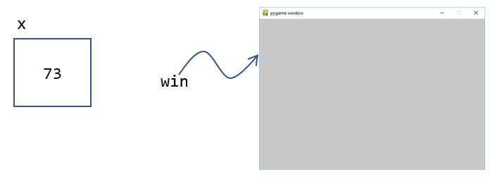
| An object in Python is a value (not unlike an integer or a float) that contains functions for accessing the data in the object. Functions associated with objects are called methods. |
For example, the Pygame window above has two methods get_height() and get_width() that return the height and width in pixels of the window. Methods are always called using a dot notation of the object name followed by the methods. For example, win.get_height().
Can you think of a way we might be able to pause the program to keep the Pygame display window from disappearing until the user hits a key on the keyboard?
The input function waits for the user to type something on the keyboard and hit enter.
1
2
3
4
import Pygame
pygame.init()
win = pygame.display.set_mode((600,600))
dummy = input("Hit <enter> to quit.") (1)
| 1 | We don’t need the dummy variable since we aren’t going to use what the user typed. We could have just said … |
input("Hit <enter> to quit.")2.1. Colors
Before we talk about drawing shapes on the window we need to know how to represent a color. A common color scheme is called RGB, for Red-Green-Blue. In Pygame a color is a triple of three values where (0,0,0) represents black all the way up to (255,255,255) which is white. There are roughly 16 million different colors we can represent. Red is (255,0,0), green is (0,255,0), and blue is (0,0,255). Yellow is red and green, so that would be (255,255,0).
| There are many online tools to help determine the RGB values for various colors. Most development environments have one too. Just do an internet search for RGB colors, or color picker.[4] |
One common thing many of our Pygame programs will do is to define some colors.
1
2
3
4
5
6
7
8
9
10
11
12
# file color.py
red = (255,0,0)
green = (0,255,0)
blue = (0,0,255)
yellow = (255,255,0)
white = (255,255,255)
black = (0,0,0)
aqua = (0,255,255)
burntsienna = (138,54,15)
lightgray = (200,200,200)
pink = (255, 20, 147)
darkgray = (100,100,100)
We will soon get tired of retyping color definitions in our Pygame programs. We can place these definitions in their own file and name it color.py.
We can then import color.py into our Pygame program with import color and voila! we have created our own Python module named color and we can reuse our color definitions without having to retype them every time.
| Put commonly used code in a separate file and import that file into each program that needs it. This allows you to reuse code you have already written rather than duplicate it. |
Don’t name your Python programs the same name as modules you commonly import. For example, if you name your program pygame.py and then in your program you have import pygame you are in the embarrassing situation of your program trying to import itself.
|
1
2
3
4
5
6
7
8
9
10
import color # this is the color.py file we just wrote above
import pygame
pygame.init()
width = 600
height = 500
win = pygame.display.set_mode((width,height)) (1)
win.fill(color.burntsienna) (2)
pygame.display.update() (3)
input("Hit <enter> to quit.") (4)
| 1 | win (short for window) is a display surface in pygame. We did not have to call it win. We could have called it any legal variable name. |
| 2 | Our first Pygame drawing command win.fill takes one argument that is an RGB color triple and fills the window with the color burntsienna from our color module. |
| 3 | When Pygame functions draw on the display the window is not actally updated until we call the Pygame function pygame.display.update(). |
| 4 | Wait for the user to hit enter so the window doesn’t disappear right away. |
2.2. Shapes
In this section we learn how to draw basic shapes; a circle, ellipse, rectangle, line, and a single pixel on a surface.
2.2.1. Rectangle
The Pygame function pygame.draw.rect draws a rectangle on a surface and takes either three or four arguments.
| Pygame programs only ever have one display surface. We will see later on that our Pygame programs may have multiple surfaces (such as an image) that we will render on a display surface. |
pygame.draw.rect(surface, color, xywh, optional-line-width)
- surface
-
The surface we are going to draw the rectangle on. For now we will just use the display surface
winthat was constructed using theset_modefunction. - color
-
An RGB triple such as (0, 255, 255) or
color.yellow(from our color module) - xywh
-
A four tuple (quadruple) that represents the \(x\) and \(y\) coordinate of the upper left hand corner of the rectangle and the width \(w\) and the height \(h\) of the rectangle. All units are in pixels.
- optional-line-width
-
If this argument is left off then the rectangle is filled in with the specified color. If it is specified then it takes a width, in pixels, of the border of the rectangle.
The upper left coordinate of a Pygame surface is the origin (0,0).
|
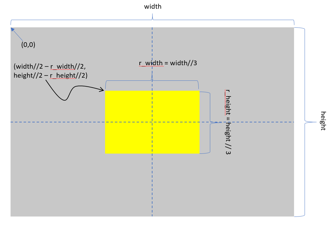
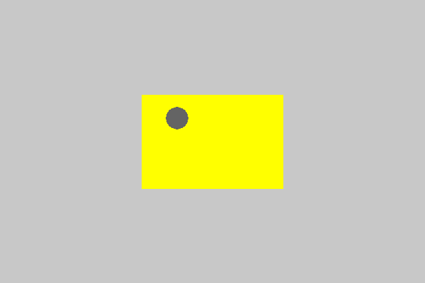
Place a yellow rectangle that is one third the width of the display surface and one third the height in the center of the display. Hint: draw this out on a sheet of paper. It is a little trickier than you think. Here is a diagram to get you started.
1
2
3
4
5
6
7
8
9
10
11
12
13
14
15
16
17
18
import pygame, color
pygame.init()
width = 600 # display surface 600 pixels wide
height = 400 # display surface is 400 pixels high
win = pygame.display.set_mode((width,height))
win.fill(color.lightgray)
# set up some variable for the rectangle
r_width = width//3
r_height = height//3
r_x = width//2 - r_width//2
r_y = height//2 - r_height//2
pygame.draw.rect(win, color.yellow, (r_x,r_y,r_width,r_height))
pygame.display.update()
input("Hit <enter> when done")
Notice the use of integer division //. All of the Pygame functions take integer arguments. Intuitively, when calculating dimensions or coordinates it doesn’t make sense to do this in fractions of a pixel.
Assume we have a 600 X 400 Pygame display.
What is the coordinate of the top left pixel in the Pygame window?
(0,0)
What is the coordinate of the top right pixel in the Pygame window?
(599,0)
Now, most likely what you said was (600,0). This is a common mistake, Remember the window is 600 pixels wide and we are starting counting at 0. So the 600th pixel is column 599. This mistake of being off by one, computer scientists quite literally call an off by one error.
What is the coordinate of the bottom left pixel in the Pygame window?
(0,399)
What is the coordinate of the bottom right pixel in the Pygame window?
(599,399)
The yellow square is proportional and relative to the size of the main Pygame display surface. That is, if we change the size of the main display surface the yellow square will resize accordingly. Most often this is the kind of graphics that we want and is one of the powerful features of doing graphics using geometric shapes. The name for this kind of graphics, using geometric shapes, is vector graphics.
| Try and always use proportional graphics. In proportional graphics a shape is drawn relative to some enclosing shape. For example, the head might be drawn relative to the window and an eye would be drawn relative to a head. A pupil would be drawn relative to the eye. If we were drawing a house, a door’s dimensions would be relative to the house’s dimensions. |
Contrast this with using absolute dimensions and absolute pixel coordinates. For example, if we draw a yellow rectangle at coordinate (100,200) with a width of 300px and a height of 200px.
pygame.draw.rect(win, color.yellow, (100,200,300,200))then this would draw the same sized yellow rectangle in the same place no matter if our display was 400 X 400 or 1000 X 1000. Worse yet if the display was 200 x 200 the yellow square would not even fit in the display.
Graphics using individual pixels only called raster graphics.
2.2.2. Circle
The Pygame function pygame.draw.circle draws a circle on a surface and takes either four or five arguments.
pygame.draw.circle(surface, color, xy, radius, optional-line-width)
- surface
-
The surface we are going to draw the rectangle on.
- color
-
An RGB triple
- xy
-
A tuple that represents the \(x\) and \(y\) coordinate of the center of the circle.
- optional-line-width
-
If this argument is left off then the circle is filled in with the specified color. If it is specified then it takes a width, in pixels, of the border of the circle.
Lets draw a dark gray circle centered in the upper left quadrant of the yellow square. We will do this proportionally, making the diameter of the circle 1/3 width of the quadrant. Calculating the x and y coordinates of the circle can be a little tricky. The width of the quadrant is r_width//2
The \(x\) coordinate of the circle is relative to r_x, the \(x\) coordinate of the yellow rectangle. Add in 1/2 the width of the quadrant you get
ul_c_x = r_x + r_width//4 # ul_c_x is short for upper left circle x coordinateSimilarly the \(y\) coordinate is
ul_c_y = r_y + r_height // 4Remember that the circle function requires the radius, but the problem stated that the
diameter of the circle is 1/3 the width of the quadrant. We know the width of the quadrant is r_width//2 and 1/3 of that is r_width//2//3 and a radius is still 1/2 of that, so we are left with
ul_c_radius = r_width//2//3//2 # or r_width // 12Defining a new color darkgray = (100,100,100) in our color module and putting it all together we have
1
2
3
4
ul_c_x = r_x + r_width // 4
ul_c_y = r_y + r_height // 4
ul_c_radius = r_width//2//3//2
pygame.draw.circle(win, color.darkgray, (ul_c_x,ul_c_y), ul_c_radius)
And we should get something that looks like
Draw another dark gray circle with the same radius centered in the upper right quadrant of the yellow rectangle.
The only thing that changes is the \(x\) coordinate. The \(y\) coordinate and the radius of the upper right circle are the same as the \(y\) coordinate and radius f the upper left circle. One way to think about the \(x\) coordinate is that it is 3/4 of the width of the rectangle.
1
2
3
4
ur_c_x = r_x + 3*r_width//4
ur_c_y = r_y + r_height // 4 # same as upper left circle
ur_c_radius = r_width//2//3//2 # same as upper left circle
pygame.draw.circle(win, color.darkgray, (ur_c_x, ur_c_y), ur_c_radius)
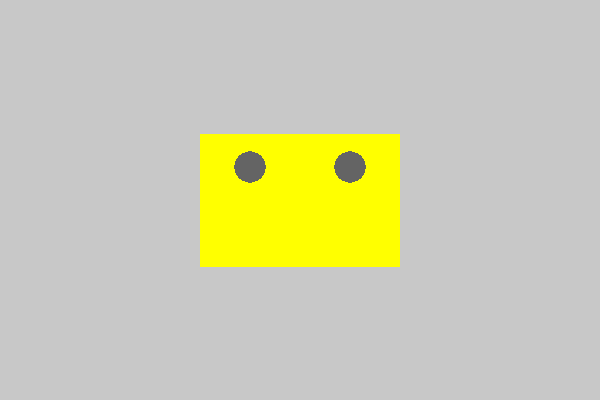
Here is the complete program so far with the two circles in the rectangle.
pygame.init()
width = 600   # display surface 600 pixels wide
height = 400  # display surface is 400 pixels high
win = pygame.display.set_mode((width,height))

win.fill(color.lightgray)

# set up some variable for the rectangle
r_width = width//3
r_height = height//3
r_x = width//2 - r_width//2
r_y = height//2 - r_height//2
pygame.draw.rect(win, color.yellow, (r_x,r_y,r_width,r_height))

ul_c_x = r_x + r_width // 4
ul_c_y = r_y + r_height // 4

# width of quadrant is r_width//2 then 1/3 of that is
# the diameter, then 1/2 of that for the radius
ul_c_radius = r_width//2//3//2
pygame.draw.circle(win, color.darkgray, (ul_c_x,ul_c_y), ul_c_radius)

ur_c_x = r_x + 3 * r_width // 4
ur_c_y = r_y + r_height // 4
ur_c_radius = r_width//2//3//2  # or r_width//12
pygame.draw.circle(win, color.darkgray, (ur_c_x,ur_c_y), ur_c_radius)

pygame.display.update()

input("Hit <enter> when done")|
Notice the line for calculating the \(x\)-coordinate of the upper right circle ur_c_x = r_x + 3 * r_width // 4 where we specified that it is three-fourths the width of the rectangle. You might be tempted to write ur_c_x = r_x + 3 // 4 * r_width Why is the incorrect? Because |
2.2.3. Ellipse
An ellipse is an oval shape with a width and a height. In graphics an ellipse is very similar to a rectangle. In fact the function to draw an ellipse is almost exactly the same as the function to draw a rectangle. The one part of drawing an ellipse that takes
some getting used to is that the (x,y) coordinate of the ellipse is the (x,y) coordinate of the rectangle (or bounding box) that surrounds the ellipse.
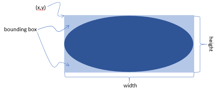
| The bounding box is the invisible rectangle that circumscribes a geometric shape such as an ellipse, circle, or polygon. |
pygame.draw.ellipse(surface, color, xywh, optional-line-width)
- surface
-
The surface we are going to draw the ellipse on.
- color
-
An RGB triple.
- xywh
-
A four tuple (quadruple) that represents the \(x\) and \(y\) coordinate of the upper left hand corner bounding box, and the width \(w\) and the height \(h\) of the ellipse.
- optional-line-width
-
same as rectangle and circle functions.
These are, in fact, the same arguments for drawing a rectangle.
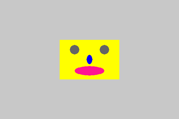
Continuing our program from before, lets draw a pink ellipse centered in the x axis, 3/4 the width of the rectangle and two-thirds of the way down the height of the rectangle. Add pink = (255, 20, 147) to our color.py module.
1
2
3
4
5
e_width = r_width // 2
e_height = r_height // 4
e_x = r_x + r_width // 2 - e_width // 2
e_y = r_y + 2 * r_height // 3
pygame.draw.ellipse(win, color.pink, (e_x,e_y,e_width,e_height))
Adding this code to our running example we should get something like …
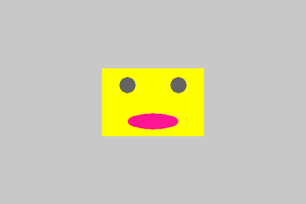
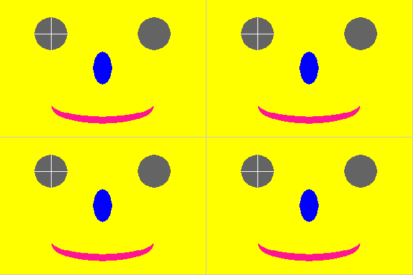
You have probably guessed by now that what is taking shape is a face, a Mr. or Mrs. Blockhead.
Use an ellipse to add a nose above the mouth.
There are lots of ways to do this, but you need to make it relative to the head.
1
2
3
4
5
n_width = r_width // 10 # 1/10th width of head
n_height = r_height // 4 # 1/4 height of head
n_x = r_x + r_width // 2 - n_width // 2 # centered horizontally
n_y = r_y + r_height // 2 - n_height//2 # centered vertically
pygame.draw.ellipse(win, color.blue, (n_x,n_y,n_width,n_height))
You can give the Blockhead a smile by drawing an ellipse over the top of the mouth shifted up slightly, and make it the same color as the background head.
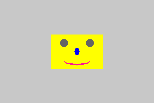
This is one line, drawing an ellipse shifted up, say 20% of the width of the mouth.
1
pygame.draw.ellipse(win, color.yellow, (e_x, e_y, e_width, e_height - .2*e_height))
Give the Blockhead pupils by drawing a circle or ellipse in each eye. Make sure it is proportional!
| You can always check to see if you are making your shapes proportional if you change the dimensions of the Pygame display at the start of the program and make sure the image resizes appropriately. |
2.2.4. Lines
You can draw a line in Pygame using the function pygame.draw.line.
pygame.draw.line(surface, color, start-xy, end-xy, optional-line-width)
- surface
-
The surface we are going to drawing the line on.
- color
-
An RGB triple
- start-xy
-
The \((x,y)\) coordinate of one endpoint of the line
- end-xy
-
The \((x,y)\) coordinate of the other endpoint of the line
- optional-line-width
-
The width of the line in pixels
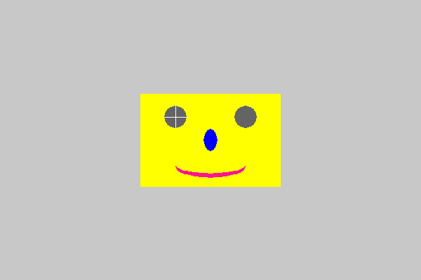
Draw a cross through the left eye.
1
2
3
4
5
6
7
pygame.draw.line(win, color.white,
(ul_c_x, ul_c_y - ul_c_radius),
(ul_c_x, ul_c_y + ul_c_radius))
pygame.draw.line(win, color.white,
(ul_c_x - ul_c_radius, ul_c_y),
(ul_c_x + ul_c_radius, ul_c_y))
There are other Pygame drawing functions that we will introduce as needed. You can make an astonishing number of drawing from rectangles, circles, ellipses, and lines.
Variables have been renamed to be more meaningful. For example, ul_c_x which stood for (upper left circle x coordinate) is now left_eye_x and so on.
import pygame, color

# initial pygame stuff
pygame.init()
width = 600   # display surface 600 pixels wide
height = 400  # display surface is 400 pixels high
win = pygame.display.set_mode((width,height))

# create the background
win.fill(color.lightgray)

# set up some variable for the head
head_width = width // 3
head_height = height // 3
head_x = width // 2 - head_width // 2
head_y = height // 2 - head_height // 2
pygame.draw.rect(win, color.yellow, (head_x, head_y, head_width, head_height))

# left eye
left_eye_x = head_x + head_width // 4
left_eye_y = head_y + head_height // 4
left_eye_r = head_width // 2 // 3 // 2  # width of quadrant is r_width//2 then 1/3 of that
pygame.draw.circle(win, color.darkgray, (left_eye_x, left_eye_y), left_eye_r)

# left eye cross
pygame.draw.line(win, color.white,
                 (left_eye_x, left_eye_y - left_eye_r),
                 (left_eye_x, left_eye_y + left_eye_r))

pygame.draw.line(win, color.white,
                 (left_eye_x - left_eye_r, left_eye_y),
                 (left_eye_x + left_eye_r, left_eye_y))

# right eye
right_eye_x = head_x + 3 * head_width // 4
right_eye_y = head_y + head_height // 4
right_eye_r = head_width // 2 // 3 // 2  # width of quadrant is r_width//2 then 1/3 of that
pygame.draw.circle(win, color.darkgray, (right_eye_x, right_eye_y), right_eye_r)

# mouth
mouth_width = head_width // 2
mouth_height = head_height // 4
mouth_x = head_x + head_width // 2 - mouth_width // 2
mouth_y = head_y + 2 * head_height // 3
pygame.draw.ellipse(win, color.pink, (mouth_x, mouth_y, mouth_width, mouth_height))

# smile
pygame.draw.ellipse(win, color.yellow, (mouth_x, mouth_y, mouth_width, mouth_height - .2 * mouth_height))

# add a nose
nose_width = head_width // 10  # 1/10th width of head
nose_height = head_height // 4 # 1/4 height of head
nose_x = head_x + head_width // 2 - nose_width // 2  # centered horizontally
nose_y = head_y + head_height // 2 - nose_height // 2  # centered vertically
pygame.draw.ellipse(win, color.blue, (nose_x, nose_y, nose_width, nose_height))

pygame.display.update()

input("Hit <enter> when done")
include:python/blockhead.pyComplete the Blockhead adding ears, hair, a hat. Make sure it stays proportional.
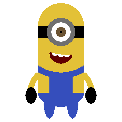
2.2.5. Sample Blockheads
To give you some ideas here are some of the blockheads that have been turned in over the years as assignments.[5]


2.3. Exercises
Answer questions about the following code fragment.
1
2
3
4
5
6
7
8
9
10
import color # this is the color.py file we just wrote above
import pygame
pygame.init()
width = 600
height = 500
win = pygame.display.set_mode((width,height))
win.fill(color.burntsienna)
pygame.display.update()
input("Hit <enter> to quit.")
-
In the statement
win.fill(color.burntsienna),winis an example of a/an (choose the best answer)-
variable
-
object reference
-
function
-
method
-
module
-
-
In the statement
win.fill(color.burntsienna),fillis an example of a/an (choose the best answer)-
variable
-
object reference
-
function
-
method
-
module
-
-
In the statement
pygame.display.update(),updateis an example of a/an (choose the best answer)-
variable
-
object reference
-
function
-
method
-
module
-
-
In the statement
pygame.display.update(),pygameis an example of a/an (choose the best answer)-
variable
-
object reference
-
function
-
method
-
module
-
So far we have encountered six different kinds of Python values. For example, integers are one. Name the others.
integers, floating-point numbers, strings, None, tuples, and object references
Write a Python/pygame program that reproduces the smiley below.

3. Functions
Functions play a massively important role in programming. They encapsulate common computations and keep programmers from having to reinvent the wheel.
You can just use the math.sqrt function. You don’t have to write it yourself.
Recall that in mathematics a function maps values in a domain to values in a range. In Python the math.sqrt function maps 4 to 2.0, 9 to 3.0, and 2 to 1.4142135623730951.[6]
math.sqrt functionThe round function maps round(3.56,1) to 3.6. Functions return values. Always. But sometimes we don’t care about the return value. In Python functions sometimes return the special value None, which essentially means the function does not "really" return a value.[7]. For example, the print function returns the value None but has the side effect of printing its arguments on the console.
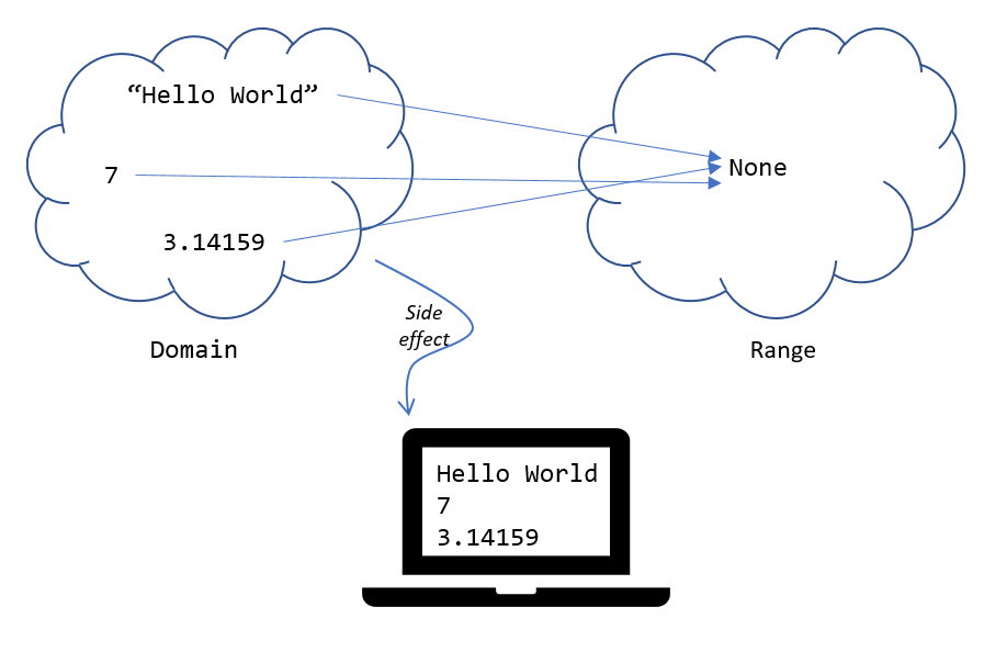
print functionWe saw earlier that
1
print("Hello World")
will print Hello World on the console, but print also returned the None value.
The following looks strange, but is legit, and almost certainly not what was intended.
1
print(print("Hello World"))
What would get printed by the code above?
1
2
Hello World
None
The inner print prints Hello World to the console and returns None to the outer print, which it prints the console. Again, strange, and almost certainly not what was intended.
None is an actual value in Python like 3 and 3.14, "Hello", and 'Goodbye'. It is the value that means no value. You will rarely ever use it explicitly.
|
3.1. Calling Functions
Lets get a little more formal about calling functions. Consider the statement
print("Hello World")We say that we are calling the print function and passing the argument Hello World. Passing an argument means we send the value to the function.
Consider our previous program where we needed to compute \(sin(\sqrt{\pi/4})\) …
1
2
result = math.sin(math.sqrt(math.pi/4))
print(round(result, 2))
How many function calls are there in the two lines above? Explain all of the arguments and return values.
The first line contains two function calls. First math.sqrt is called with the argument math.pi/4. Then math.sin is called and uses the value returned from the math.sqrt call as its arguments. The return value of math.sin is then assigned to the variable result. The second line contains two function calls as well. First round is called with two arguments, result and 2. result is the value being rounded and 2 is the number of places to round to. The return value from round is then used as the only argument to the print function.
In total there are four function calls and five arguments involved.
3.2. Defining Functions
The real power with functions is that programmers get to define our own. Functions allow us to encapsulate commonly occurring computations. Lets go back to our rather banal example of our formula to convert a Fahrenheit temperature to Celsius. Rather than having to keep remembering the formula we can just define a function.
1
2
3
def f2c(f): (1)
c = 5 / 9 * (f - 32) (2)
return c (3)
| 1 | This is the function header. It tells Python we are defining our own function and it takes one parameter f. The value of f is determined by the argument when f2c is called. |
| 2 | This is the main part of the function that does the computation. It defines a local variable c. |
| 3 | This is the return statement that indicates that function f2c returns the value c to the caller that was just computed. |
Lines 2 and 3 constitute the function body, which is indented under the function header.
We now have our own function for converting Fahrenheit to Celsius and we can tuck it away in a file somewhere so we can reuse it later.
We can use f2c in a program by calling it with an argument.
print(f2c(32))We call this the main program. The main program is any code that exists outside of a function.
Why is the following line incorrect?
f2c(32)
Because f2c returns a value, and this line does not do anything with that value. It doesn’t print it or use it in another computation.
It is a common mistake for students to confuse a function returning a value and a function printing a value. Consider this version of f2c.
1
2
3
def f2c(f):
c = 5 / 9 * (f - 32)
print(c)
This function returns the value None and, as a side effect, prints the value of the variable c on the console. This function is not technically wrong. It does not have a syntax error, nor a run-time error, or even a logic error. But it is in some way inferior to the first version of f2c. Consider the following program.
1
2
t = float(input("Enter a temperature: "))
print(f2c(t) + 100)
This program reads a temperature from the user and puts it in the variable t. It then converts t to Celsius and adds 100 degrees Celsius to the result and printing the final value. For the first version of f2c this works fine. But the second version crashes because it tries to add 100 to None.
| A function that returns a value is not the same thing as the function printing a value. |
3.3. Functions for their side effect
Functions return values. Some functions, such as print, return None but are used for their side effect.
Recall our complete blockhead program from before.
import pygame, color

# initial pygame stuff
pygame.init()
width = 600   # display surface 600 pixels wide
height = 400  # display surface is 400 pixels high
win = pygame.display.set_mode((width,height))

# create the background
win.fill(color.lightgray)

# set up some variable for the head
head_width = width // 3
head_height = height // 3
head_x = width // 2 - head_width // 2
head_y = height // 2 - head_height // 2
pygame.draw.rect(win, color.yellow, (head_x, head_y, head_width, head_height))

# left eye
left_eye_x = head_x + head_width // 4
left_eye_y = head_y + head_height // 4
left_eye_r = head_width // 2 // 3 // 2  # width of quadrant is r_width//2 then 1/3 of that
pygame.draw.circle(win, color.darkgray, (left_eye_x, left_eye_y), left_eye_r)

# left eye cross
pygame.draw.line(win, color.white,
                 (left_eye_x, left_eye_y - left_eye_r),
                 (left_eye_x, left_eye_y + left_eye_r))

pygame.draw.line(win, color.white,
                 (left_eye_x - left_eye_r, left_eye_y),
                 (left_eye_x + left_eye_r, left_eye_y))

# right eye
right_eye_x = head_x + 3 * head_width // 4
right_eye_y = head_y + head_height // 4
right_eye_r = head_width // 2 // 3 // 2  # width of quadrant is r_width//2 then 1/3 of that
pygame.draw.circle(win, color.darkgray, (right_eye_x, right_eye_y), right_eye_r)

# mouth
mouth_width = head_width // 2
mouth_height = head_height // 4
mouth_x = head_x + head_width // 2 - mouth_width // 2
mouth_y = head_y + 2 * head_height // 3
pygame.draw.ellipse(win, color.pink, (mouth_x, mouth_y, mouth_width, mouth_height))

# smile
pygame.draw.ellipse(win, color.yellow, (mouth_x, mouth_y, mouth_width, mouth_height - .2 * mouth_height))

# add a nose
nose_width = head_width // 10  # 1/10th width of head
nose_height = head_height // 4 # 1/4 height of head
nose_x = head_x + head_width // 2 - nose_width // 2  # centered horizontally
nose_y = head_y + head_height // 2 - nose_height // 2  # centered vertically
pygame.draw.ellipse(win, color.blue, (nose_x, nose_y, nose_width, nose_height))

pygame.display.update()

input("Hit <enter> when done")
include:python/blockhead.py
What if we wanted to draw two or more blockheads on the display surface? One way is to make another copy of the code, and change lots of variable names etc. This is a perfect situation where we can write a function blockhead that we can call more than once.
In keeping with the way drawing rectangle works specifying the Blockhead’s \(x\) and \(y\) coordinate along with its width and height makes sense:
1
2
def draw_blockhead(head_x, head_y, head_w, head_h):
pass
This is just the function header. The Python statement pass is the statement that does nothing. We are using it here as a placeholder for the function body, which we have not yet written.
So what we’ll do now is place all of the code used for the drawing inside the function and make sure that we use the parameters to initialize the
1
2
3
4
5
6
7
8
9
10
11
12
13
14
15
16
17
18
19
20
21
22
23
24
25
26
27
28
29
30
31
32
33
34
35
36
37
38
39
40
41
42
43
44
45
46
47
48
def draw_blockhead(head_x, head_y, head_w, head_h):
pygame.draw.rect(win, color.yellow,
(head_x, head_y, head_width, head_height))
# left eye
left_eye_x = head_x + head_width // 4
left_eye_y = head_y + head_height // 4
left_eye_r = head_width // 12
pygame.draw.circle(win, color.darkgray,
(left_eye_x, left_eye_y), left_eye_r)
# left eye cross
pygame.draw.line(win, color.white,
(left_eye_x, left_eye_y - left_eye_r),
(left_eye_x, left_eye_y + left_eye_r))
pygame.draw.line(win, color.white,
(left_eye_x - left_eye_r, left_eye_y),
(left_eye_x + left_eye_r, left_eye_y))
# right eye
right_eye_x = head_x + 3 * head_width // 4
right_eye_y = head_y + head_height // 4
right_eye_r = head_width // 12
pygame.draw.circle(win, color.darkgray,
(right_eye_x, right_eye_y), right_eye_r)
# mouth
mouth_width = head_width // 2
mouth_height = head_height // 4
mouth_x = head_x + head_width // 2 - mouth_width // 2
mouth_y = head_y + 2 * head_height // 3
pygame.draw.ellipse(win, color.pink,
(mouth_x, mouth_y, mouth_width, mouth_height))
# smile
pygame.draw.ellipse(win, color.yellow,
(mouth_x, mouth_y, mouth_width, mouth_height - .2 * mouth_height))
# add a nose
nose_width = head_width // 10 # 1/10th width of head
nose_height = head_height // 4 # 1/4 height of head
nose_x = head_x + head_width // 2 - nose_width // 2
nose_y = head_y + head_height // 2 - nose_height // 2
pygame.draw.ellipse(win, color.blue,
(nose_x, nose_y, nose_width, nose_height))
Now we can call the draw_blockhead function as many times as we like without having to
duplicate lots of code. The variables head_x, head_y, head_w, head_h are parameters and they can be used anywhere in the function body. That is their scope.
| The scope of a variable is the region of the program where it can be used. |
All of the other variables that are defined in the function are local variables. A local variable’s scope is from the point where where it is defined until the end of the function.
| A local variable is defined in a function. Its scope is the point from where it was defined until the end of the function. |
The draw_blockhead function still uses the variable win, which is neither passed as a parameter nor is it defined with the function. The function assumes win is defined in the main program. We say that win is a global variable.
| A global variable is defined in the main program. Its scope is the point from where it was defined until the end of the program. |
1
2
3
4
5
6
7
8
9
10
11
12
13
14
15
16
17
18
# initial Pygame stuff
import pygame, color
pygame.init()
width = 600 # display surface 600 pixels wide
height = 400 # display surface is 400 pixels high
win = pygame.display.set_mode((width,height))
# create the background
win.fill(color.lightgray)
blockhead(0,0,299,199)
blockhead(300,0,299,199)
blockhead(0,200,299,199)
blockhead(300,200,299,199)
pygame.display.update()
input("Hit <enter> when done")
3.4. Benefits of functions
3.4.1. Functions make code more readable
If you look at the main program above it is clear that the program draws four figures. If we didn’t use a function and duplicated the code to draw the figures then it would be far less clear what is going on.
3.4.2. Functions make code less buggy
Imagine had we not used a function and we found an error in the code, we would then have to fix that error in every place where the code was duplicated. When we use a function we just fix it once.
3.5. Exercises
Write a function circ_area that that takes the radius of a circle as a parameter and returns the area of the circle. Write a main program that reads the radius from the user (keyboard) and prints the area.
Answer questions about the program below.
1
2
3
4
5
6
7
8
9
10
11
12
x = 5
y = 6
z = 33
def f(x):
y = 9
print(x + y + z)
print(x + y + z)
f(12)
print(x + y + z)
pass
-
What is the output of the program?
-
Which line contains a function header?
-
Which line(s) constitute the main program?
-
Is there a local variable defined anywhere? If so what is its scope?
-
Does the function
freturn a value? -
Does the function
freference any global variables? -
Which lines constitute a function body?
-
Are there any arguments used in the program? If so what and where are they? (tricky)
-
Are there any parameters defined in the program? Explain.
-
What does the last line do?
What is a built-in function?
Assume that C is an initial amount of an investment, r is the yearly rate of interest (e.g., .02 is 2%), t is the number of years until maturation, n is the number of times the interest is compounded per year, then the final value of the investment is \(p=c(1+r/n)^{tn}\). Write a function investment that takes C, r, n, and t as arguments and returns the final value of the investment to the nearest penny. Test your function with a main program where \(C = 1000, r = .01, n = 1, t = 1\).
This exercise should be familiar from Chapter 1.
def investment(c,r,n,t):
    p = c*(1 + r/n)**(t*n)
return p (1)| 1 | We didn’t have to use the local variable p. We could just as well have said return c*(1 + r/n)**(t*n) |
Test on \(C = 1000, r = .01, n = 1, t = 1\).
print(interest(1000,.01,1,1)) (1)| 1 | Should print 1010.0 |
4. Repetition - The While Loop
Lets assume we have a particle (a circle, face, or image of a ball).[8] on a Pygame display surface drawn halfway down the display and all the way to the left.
| We will often use the term particle to represent a moving object such as a baseball, a hockey puck, an electron, etc. The term particle comes from physics and is an abstract representation of some object. |
When the particle is obviously something like a soccer ball I will often use the term particle and ball interchangeably.
1
2
3
4
5
6
7
8
9
10
11
12
13
14
15
import color, pygame
pygame.init()
side = 500
win = pygame.display.set_mode((side,side))
# properties of the particle
radius = side//20
px = radius # particle is all the way to the left (1)
py = side//2 # and halfway down display
win.fill(color.white)
# draw the particle
pygame.draw.circle(win, color.blue, (px, py), radius)
pygame.display.update()
| 1 | Where would the particle show up of we set px = 0 |
What if we wanted to draw another particle right next to the first? The next particle’s \(x\) coordinate will be one diameter (or 2 radii) past the first particle’s \(x\) coordinate.
1
2
px = px + 2 * radius
pygame.draw.circle(win, color.blue, (px, py), radius)
How about a third particle?
1
2
px = px + 2 * radius
pygame.draw.circle(win, color.blue, (px, py), radius)
And a fourth particle? … well, you get the picture. We could keep copying and pasting until we have as many particles displayed as we need. This should feel wrong. And it is. What we want to do is repeat those two lines until the display is filled with particles.

The while loop repeats a body of code (indented) as long as some condition is true. The syntax is …
while (condition):
    stmt
We want to keep repeating the two lines of code
1
2
px = px + 2 * radius
pygame.draw.circle(win, color.blue, (px, py), radius)
as long as some condition is true. In this case, as long as the particle’s right edge is to the left of the right edge of the display.
1
2
3
while px + radius < side:
px = px + 2 * radius
pygame.draw.circle(win, color.blue, (px, py), radius)
Eventually px + radius will become greater than side and the loop condition becomes false and then the loop terminates.
Note: True and False are values in Python, just like the integer 1 and the float 3.14159. True an False are called boolean values.
4.1. Animation
One modification is that we can animate the particle moving across the screen smoothly. Rather than redraw the particle two radii, shift the particle by just one pixel. We can also add a delay. Finally, before we redraw the particle we can erase the display. This is a standard way of animating an object in computer graphics:
-
Erase the background
-
Update the object’s position (for example, the particle’s \(x\)-coordinate).
-
Redraw the object
-
introduce a slight delay to model (mimic or simulate) the passage of time
1
2
3
4
5
6
while px + radius < side:
win.fill(color.white) (1)
pygame.draw.circle(win, color.blue, (px,py), radius)
pygame.display.update()
pygame.time.delay(5) (2)
px = px + 1 (3)
| 1 | erase the screen, effectively erasing the particle |
| 2 | delay 5 milliseconds |
| 3 | moving 1 pixel at a time makes the motion look smooth |
| A sprite is a more general computer graphics term for a 2-dimensional object that is animated in a larger scene. Our particle is an example of a sprite. |
4.2. Relational Operators
So far we have only used the less than relational operator < that compares two values. Table Relational Operators lists them all.
| Operator | operation |
|---|---|
|
less than |
|
less than or equal to |
|
greater than |
|
greater than or equal to |
|
equal to |
|
not equal to |
Animate moving the particle to the bottom of the screen.
While the particle’s \(y\)-coordinate plus the radius is less than the side length.
1
2
3
4
5
6
while py + radius < side: (1)
win.fill(color.white)
pygame.draw.circle(win, color.blue, (px,py), radius)
pygame.display.update()
pygame.time.delay(5)
py = py + 1
| 1 | What would happen if we simply had while py < side? |
Animate moving the particle from right to left.
While the particle’s \(x\)-coordinate is greater than 0.
1
2
3
4
5
6
while px > 0:
win.fill(color.white)
pygame.draw.circle(win, color.blue, (px,py), radius)
pygame.display.update()
pygame.time.delay(5)
px = px - 1
Animate moving the particle to the top of the screen.
While the particle’s \(y\)-coordinate is greater than 0.
1
2
3
4
5
6
while py > 0:
win.fill(color.white)
pygame.draw.circle(win, color.blue, (px,py), radius)
pygame.display.update()
pygame.time.delay(5)
py = py - 1
| Whenever you find yourself copying and pasting the same lines of code over and over that is a sure sign that either 1) you should be encapsulating that code in a function, or 2) it should be repeating in a loop. |
4.3. Counting Loops
A common loop pattern is to repeat a body of code an exact number of times.
Lets print a table of powers of two up to 210.
i   2^i
==========
0  | 1
1  | 2
2  | 4
3  | 8
...
10 | 1024
1
2
3
4
5
6
7
8
# table header
print("i 2^i")
print("=========")
i = 0 (1)
while i <= 10: (2)
print(i, '\t|', 2**i) (3)
i = i + 1 (4)
| 1 | In a counting loop we almost always initialize a variable to 0. It is a convention to use i, j, and k as a name for a counting variable. |
| 2 | We want to include 10 in our table so we use <= here. Could we have also said i < 11? Yes. |
| 3 | '\t' represents the tab character. Without it the table columns would not be lined up neatly. Recall our discussion of escape characters back in the section on string literals. |
| 4 | This increments the value of i by 1. |
Lets be careful how we interpret the statement i = i + 1. This is an assignment statement, not a statement in mathematics (which would be nonsense). The way to read this is the new value of i gets the old value of i plus one.
What would happen if we forgot the line i = i + 1?
Since i would never increment, the loop condition would never become false and the loop would never terminate. This is called an infinite loop. Furthermore,
the program would keep printing the line 0 | 1
| A convention is something that is common practice. Stick with conventions as it makes code more readable. |
Write a while-loop that prints the integers from 1 to 10, one integer per line.
Here is one way to do it.
1
2
3
4
i = 1
while i <= 10:
print(i)
i = i + 1
Does the following program work? If not, fix it.
1
2
3
4
i = 1
while i < 10:
i = i + 1
print(i)
You could fix it by starting i at 0 instead of 1.
Print the integers counting down from 10 to 0. When you are done print "Blast off!". Add a one second delay in between integers. Hint: use the pygame.time.delay(n) function where n is the number of
milliseconds to delay.
There is a 1000 milliseconds in a second.
1
2
3
4
5
6
7
8
import pygame
i = 10
while i > -1:
print(i)
i = i - 1
pygame.time.delay(1000)
print("Blast off!")
4.4. Accumulating Loops
Another common loop pattern is to keep a running total. For example, computing the sum of the integers from \(1\) to \(n\). That is, \(1 + 2 + 3 + \cdots + n\) where \(n\) is entered by the user.[9]
1
2
3
4
5
6
7
8
9
n = int(input("Enter n: "))
i = 1 (1)
total = 0 (2)
while i <= n: (3)
total = total + i (4)
i = i + 1 (5)
print("The sum from 1 to", n, "is", total)
| 1 | The loop counter. This could have started at 0, however, including 0 in the total doesn’t change the final value. |
| 2 | Keep track of the running total in total. I have purposefully avoided
usng the variable named sum because sum is also the name of a built-in function. |
| 3 | Make sure to include n |
| 4 | This adds the current value of i to the running total in total. Again, interpret this as the assignment statement the new value of total gets the old value of total plus i. |
| 5 | Increment the loop counter |
|
Programmers often use assignment statements such as |
Write a program that computes the average of non-negative numbers (e.g., quiz grades) entered by the user. Quit reading numbers when the user has entered a negative number. Be careful, make sure you don’t include the negative number in the average. Here is an example run of the program.
Enter a number: 3
Enter a number: 9
Enter a number: 7
Enter a number: 8
Enter a number: -1
The average is  6.75
1
2
3
4
5
6
7
8
9
10
11
n = float(input("Enter a number: "))
i = 0
total = 0
while n >= 0:
i += 1
total += n
n = float(input("Enter a number: "))
average = total / i
print("The average is ", round(average, 2))
This is actually a little tricky. Notice the first line. We read our first number before the loop. Once we get into the loop we know that we must have entered a non-negative number.
There is actually a subtle bug in this code that can sometimes lead to a crash. Can you find it?[11]
4.5. Exponential Growth (Example: Password Length)
Why are longer passwords better than shorter passwords? It is obvious, longer passwords are harder to guess. But how much harder? Lets say we allowed passwords to contain 26 upper or lower case characters (that is 52 possible alphabetic characters, in the English alphabet), ten digits 0 through 9, and 32 symbol characters ~!@#$%^&*()_-+={[}]"':;>.<,?/|\. That is 94 possible distinct characters that can be used in a password.[12]
There are \(94\) one character passwords, \(94^2 = 8836\) two character passwords, \(94^3 = 830584\) three character passwords, and so on, so that if a password was ten characters long there are \(94^{10} = 53861511409489970176\) possible passwords or approximately \(5 \times 10^{19}\).
Plotting \(94^i\), where \(i\) is the number of characters in the password, gives us the graph:
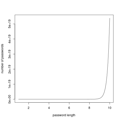
This is an example of exponential growth in the number of characters in the password. Notice how the graph explodes at between 8 and 10 characters (was it ever suggested that you make your passwords more than 8 characters long?) What is the total number of passwords up to 10 characters long? We would have to include all of the nine character passwords, and the eight character passwords, etc. and compute the sum \(94^1 + 94^2 + 94^3 + \cdots + 94^{10}\).
1
2
3
4
5
6
7
i = 1
total = 0
while i <= 10:
total += 94**i
i += 1
print(total)
which would print 54440667446151152650, which is also just bigger than \(5.4 \times 10^{19}\).
To emphasize the difference between a six character password and a ten character password, let’s assume a malicious hacker was trying to break into a system by trying all possible passwords. How long might it take? Lets say we had a powerful computer that could attempt 1 billion passwords per second.
For a six character password that’s \(94^6/10^9/60 \approx 11.5\) minutes to try all possibilities. On average we will search about half the passwords, so on average it would take about \(6\) minutes.
For a ten character password, we have \(94^{10}/10^9\) seconds. Dividing by \(60\) to get minutes then another \(60\) for hours, then \(24\) to get days, then \(365.25\) to get years, we have \(94^{10}/10^9/60/60/24/365.25 = 1706\) years! Again, this is to try them all, so on average we would find it after looking at half of the passwords, so it would only take about \(850\) years.
| A brute force attack is one where an attacker tries all possible combinations of passwords. The number of possible passwords grows exponentially with their length. As we saw, brute force attacks are most effective against short passwords. |
4.6. Exponential Growth (Example: Population)
Exponential growth arises in more subtle ways. In the previous example we were raising the base of the exponent, 94, to a fairly large power. What if the base were small, but still greater than one? Lets use an example of world population growth rate, which is currently estimated to be 1.11% (or .011) per year in 2017.[13]
Let \(t\) be the current year and \(P_t\) be the current population at the beginning of year \(t\). So \(P_{t+1} = P_t + 0.011P_t\) or, factoring out the \(P_t\) then \(P_{t+1} = P_t(1.011)\).
One way of interpreting the formula \(P_{t+1} = P_t(1.011)\) is to see that the new value of \(P\) is the old value of \(P\) times 1.011. We have seen this pattern before in code. It is just an assignment statement:
P = P * 1.011We can just keep iterating this statement after we give it an initial population.
1
2
3
4
5
P = 7.5e9 # initial population
P = P * 1.011 # population after year 1
P = P * 1.011 # population after year 2
P = P * 1.011 # population after year 3
# and so on
Of course if we want to compute the population P after \(n\) years we should use a loop.
1
2
3
4
5
6
7
8
9
10
P = 7.5e9 # initial population 7.5 billion
i = 0 # counter
r = .011 # growth rate 1.1%
n = int(input("Enter a number of years: "))
while i < n:
P = P * (1 + r)
i = i + 1
print("Final population: ", int(P))
Assume we have current population of roughly 7.5 billion.[14] If we look at plots over a 10 year (top left), 100 year (top right), 1000 year (bottom left), and 5000 year (bottom right) time horizon then the year plot looks nearly linear. But as we progress up to 5000 years we see that this seemingly linear growth is a mirage and we have a curve that is definitely exponential.
|
|
|
|
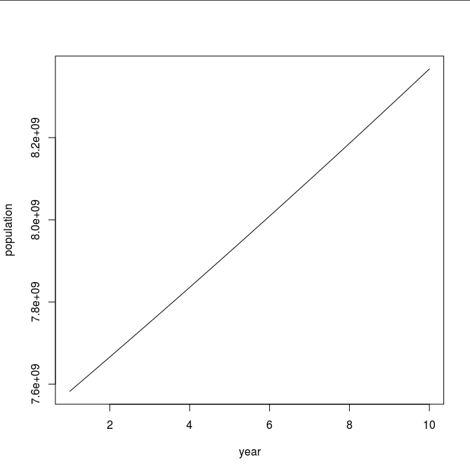
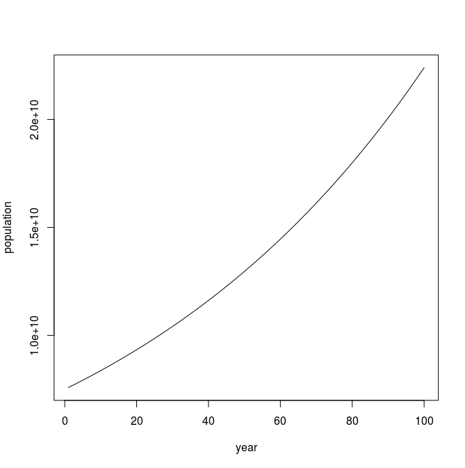
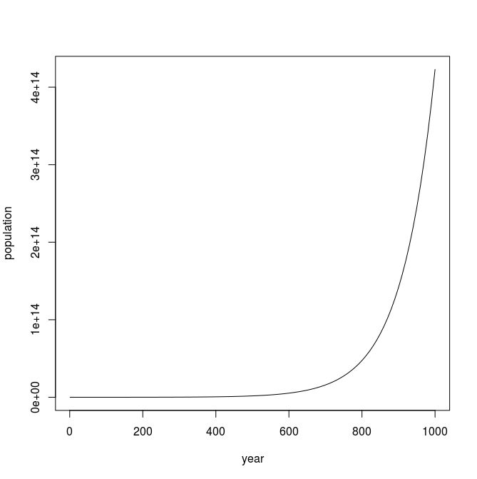
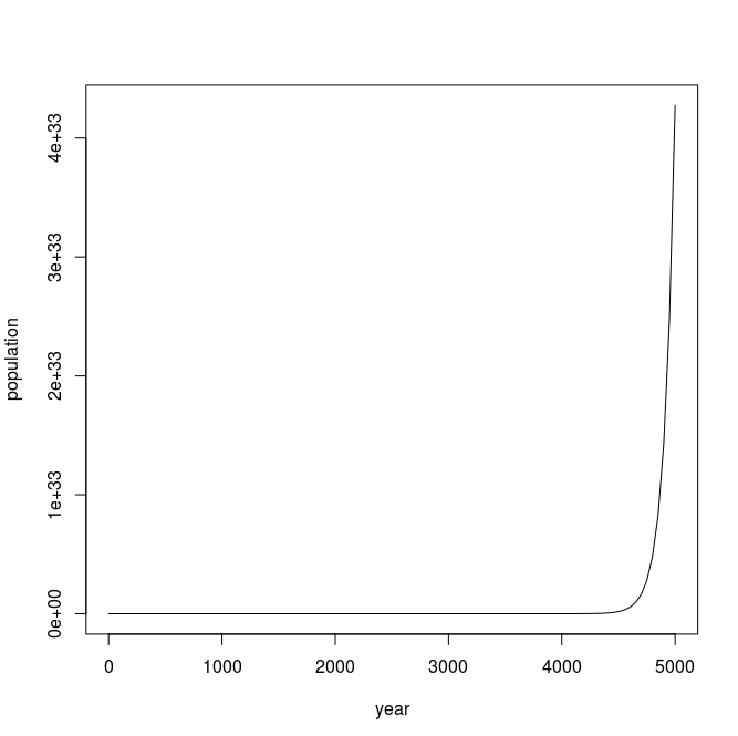
| Linear growth follows the equation of a line, \(y=mx+b\) where \(m\) is the slope and \(b\) is the \(y\)-intercept. |
| The mathematically inclined will notice that if we just keep iterating the statement \(P = P(1+r)\) we can use a little algebra and keep substituting \(P(1+r)\) for \(P\). Substituting once we get \(P = P(1+r)(1+r) = P(1+r)^2\). If we substitute a third time we get \(P = P(1+r)(1+r)(1+r) = P(1+r)^3\). After \(n+1\) substitutions we get \(P_{n+1} = P(1+r)^n\), and the exponential is obvious. |
When using a loop like this we can easily ask alternative questions such as how many years will it take to reach a population of 10 billion? This is just a simple matter of rephrasing the loop condition.
1
2
3
4
5
6
7
8
9
p = 7.5e9 # initial population 7.5 billion
i = 0 # counter
r = .011 # growth rate 1.1%
while p < 10e9:
p = p * (1 + r)
i = i + 1
print(i, "years to 10 billion")
The population growth rate is not constant. It fluctuates and has increased and decreased over the centuries. Currently it is decreasing at a rate of about .025% per year (.00025). Can we modify our program to incorporate a decreasing growth rate? The beauty of programming is that incorporating changes like this is easy compared to trying to figure out the mathematics. Below is a graph over a 50 year period beginning with our current population. After 50 years the population is approximately \(9.5 \times 10^9\).
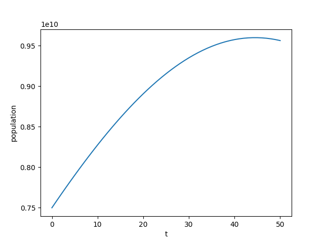
If the growth rate decreases long enough it will eventually become negative. Correspondingly, the population will start shrinking.
1
2
3
4
5
6
7
8
9
10
11
p = 7.5e9 # initial population 7.5 billion
i = 0 # counter
r = .011 # growth rate 1.1%
n = int(input("Enter a number of years: "))
while i < n:
p = p * (1 + r)
i = i + 1
r = r - .00025 (1)
print("Final population: ", int(p))
| 1 | This is the only line that has changed from the original solution. The rate decreases by .025% every year. |
4.7. Checksums; detecting network communication errors
A checksum is an integer derived from a larger integer and is used to detect communication errors in a network. There are many different checksum techniques but one of the easiest to understand is to add up the digits in a base-ten integer mod ten, and then append that number to the original integer. Recall that in a computer, everything is represented as bits; music, images, web pages, Word documents, etc. Sequences of bits are just integers. Rather than work in the language of bits, binary, 0s and 1s, we will stick with the more familiar base-ten digits 0-9.
If a network was transmitting the number \(51623\) we would compute the checksum by computing \((5+1+6+2+3)\% 10 = 7\) and we would then transmit the number \(516237\). We call \(7\) the checksum digit, or just checksum for short. What would happen if there was an error in the transmission and the number transmitted was \(596237\). We remove the checksum digit \(7\), and compute the checksum of \(59623\) which is \((5+9+6+2+3) \% 10 = 5\) and we see that \(7 \neq 5\) so there must have been an error in the transmission.
Why does this work? This only works if there is a single error in a digit. It is easy to construct a case where if there were multiple errors this would not work. For example, if we were transmitting the value \(516237\) and there were two errors in the original communication such as \(526137\) the checksum is \(7\) in both. If there is only single error it makes sense that a change in any single digit would change the final checksum mod \(10\).
What is the checksum digit for the integer \(198723\)?
It is \(0\) because \((1 + 9 + 8 + 7 + 2 + 3) \% 10 = 30 \% 10 = 0\).
How can we write a program to compute a checksum? If we have an integer such as \(51623\) we can get the last digit using \(\% 10\); for example, \(51623 \% 10 = 3\). Then we need to do the same to the remaining digits \(5162\). We can get that using integer division by 10, \(51623 // 10 = 5162\). We just keep repeating this process adding up the remainder until the number has been reduced to \(0\).
We can put this in a function that takes an integer to compute the checksum of and return the checksum.
1
2
3
4
5
6
7
def checksum(n):
total = 0
while n > 0:
total = total + (n % 10) (1)
n = n // 10 (2)
return total % 10
| 1 | or `total += n % 10 |
| 2 | or n //= 10 |
-
Does the
checksumfunction use any local variables? -
non line 1 is a ________________________ -
Line 1 is the function ________________________
-
Lines 2-7 constitute the function ________________________
-
totalon line 2 is defined as a ______________________ variable. -
What is the value of
checksum(91242)
How can we append the checksum of an integer to the end (the least significant digit)? For example if the checksum of \(51326\) is \(7\) how do we build the new integer \(513267\)?
1
2
check = checksum(x) (1)
data = x * 10 + check (2)
| 1 | Compute the checksum of x, the integer we want to transmit |
| 2 | Multiply x by 10 shifting it left, and then add in the checksum digit check. |
4.8. While-Loop Exercises
If you haven’t done the Check Yourself exercises in this chapter do those now.
The Fibonacci Sequence is the sequence of integers \(0,1,1,2,3,5,8,13\cdots\). Each Fibonacci number is the sum of the previous two Fibonacci numbers. By definition the first two Fibonacci numbers are \(0\) and \(1\). If the first Fibonacci number is \(0\) then the seventh Fibonacci number is \(8\). Write a while-loop to compute the one-hundredth Fibonacci number. Hint: This is a little tricky. Use two variables, one to keep track of the current Fibonacci number and one for the previous Fibonacci number.
The answer you get should be 218922995834555169026. This is a surprisingly large number. The Fibonacci sequence actually exhibits exponential growth.
Write a while loop to compute the sum of squares from \(1\) to \(100\), or \(1^2 + 2^2 + 3^2 + \cdots + 100^2\).
How many times will hello be printed by the code below?
1
2
3
4
i = 2
while i < 11:
print("hello")
i = i + 2
How many times will hello be printed by the code below?
1
2
3
4
i = 12
while < 18:
print("hello")
i = i + 1
What is the output the code below?
1
2
3
4
5
i = 1
n = 10
while i < n:
i = i * 2
print(i)
Write a function num_digits that will return the number of digits in an integer. For example,
if we were to call num_digits(5132981) it would return 7 because there are 7 digits in 5132981. Hint: this is similar to the checksum program.
The * operator can be applied to a string and an integer. For example, 'Z' * 5 evaluates to ZZZZZ. Write a Python program that reads an integer from the user and prints a triangle pattern of asterisks. For example, if the user enters 6 then there are six rows of asterisks where the first row has one asterisk and the sixth row has six asterisks as in the sample output below.
Enter n: 6
*
**
***
****
*****
******
1
2
3
4
5
6
n = int(input("Enter n: "))
i = 1
while i <= n:
print('*' * i) (1)
i = i + 1
| 1 | Print i asterisks and an end-of-line character. |
5. Conditionals
Lets simulate tossing a coin and print Heads or Tails with a 50-50 chance.
The random module contains many functions for generating random numbers. The function random.random() returns a uniform floating-point number between 0 and 1.
| A random number generator is uniform if all outcomes are equally likely. |
1
2
import random
print(random.random())
0.2840077963246783
The function random.randrange(n) returns a uniform random integer between 0 and n-1 inclusive.
1
2
import random
print(random.randrange(6))
We need some way to check what the random number generator produced. The if-statement executes one of two possible blocks of statements depending on a logical condition.
if (condition):
    true_stmts
else:
    false_stmts
If the condition is true then the block of statements labeled true_stmts will be executed, otherwise the block of statements labeled false_stmts will be executed. The else part is optional. if and else are new keywords. They cannot be used as variable or function names. Notice also that the statements under the if of else are indented just like a function body or the body of a while loop.
Back to simulating a coin toss. Here is one way using random.random()
1
2
3
4
5
6
7
import random
x = random.random()
if x < 0.5:
print("Heads") (1)
else:
print("Tails")
| 1 | Assigning heads to be less than .5 is, of course, arbitrary. We could have just as easily made tails be less than .5. |
Here is another way using random.randrange()
1
2
3
4
5
6
7
import random
x = random.randrange(2)
if x == 0:
print("Heads") (1)
else:
print("Tails")
| 1 | Similar to the above, assigning heads to be 0 is arbitrary. |
Using either random.random() or random.randrange() is fine. One way is not particularly better than the other. Using random.random() makes it a little easier to simulate tossing an unfair coin. For example, a coin that comes up heads two-thirds of the time.
1
2
3
4
5
6
7
import random
x = random.random()
if x < 2/3: (1)
print("Heads")
else:
print("Tails")
| 1 | If the random number generator is uniform then this should ensure that x is less than 2/3, well, with probability 2/3. |
Using random.randrange() is a little tricker, but you can come close.
1
2
3
4
5
6
7
import random
x = random.randrange(1000)
if x < 667: (1)
print("Heads")
else:
print("Tails")
| 1 | Not exactly two-thirds, but close. How can we make it more accurate? |
Write a program that reads an integer from the keyboard and prints even, if the number was even, or odd if the number was odd. A number is even if it is divisible by two. That is, the remainder after dividing by two is zero.
1
2
3
4
5
6
n = int(input("Enter an integer: "))
if n % 2 == 0:
print(n, "is even")
else:
print(n, "is odd")
5.1. if-elif-else
Lets take an example of tossing a single die [15]. We will print one if we rolled a one, two if we rolled a two, etc. One way to write this:
1
2
3
4
5
6
7
8
9
10
11
12
13
14
15
16
17
18
19
import random
d = random.randrange(6) + 1
if d == 1:
print("one")
else:
if d == 2:
print("two")
else:
if d == 3:
print("three")
else:
if d == 4:
print("four")
else:
if d == 5:
print("five")
else:
print("six")
This is pretty confusing and not very readable. Most programming languages have an alternative form of the if-statement that we sometimes call if-else-if. Here is Python’s version:
if (condition1):
    stmts1
elif (condition2):
    stmts2
elif (condition3):
    stmts3

	...

else:
    stmts_else
The final else clause is optional. Note the new keyword elif. condition1 is checked first and if it is true then stmts is executed, and the remainder of the if-elif-statement is skipped. If condition1 is false we check condition2 and so on.
Now we can write our die toss program as:
1
2
3
4
5
6
7
8
9
10
11
12
13
d = random.randrange(6) + 1
if d == 1:
print("one")
elif d == 2:
print("two")
elif d == 3:
print("three")
elif d == 4:
print("four")
elif d == 5:
print("five")
else:
print("six")
5.2. Logical Operators
Up until now our conditions in either the while loop or the if-statement have been relatively simple. Python, as do all other programming languages, allow you to state more complicated conditions such as, if the temperature greater than 50 and less than 100. We have new Python keywords and, or, not.
5.2.1. Logical and
Lets say we rolled a pair of dice and wanted to check if we rolled two ones (snake eyes). Our first attempt, might be:
1
2
3
4
5
6
d1 = random.randrange(6) + 1
d2 = random.randrange(6) + 1
if d1 == 1:
if d2 == 1:
print("snake eyes!")
This works just fine, albeit a bit clunky. More concise would be to use the logical operator and.
1
2
3
4
5
d1 = random.randrange(6) + 1
d2 = random.randrange(6) + 1
if d1 == 1 and d2 == 1: (1)
print("snake eyes!")
| 1 | and is a Python keyword. |
The logical operator and combines a logical value on the left and the right, X and Y. The entire logical expression is true if both X and Y are true. We often state this interms of a truth table.
False and True are Python keywords.
| X | Y | X and Y |
|---|---|---|
|
|
|
|
|
|
|
|
|
|
|
|
| A truth table enumerates all possible outcomes of a logical operator for all possible inputs. |
Write an if-statement that checks whether an integer n is between 0 and 100 inclusive. If it is then set a variable x to 0. Write it two ways, one using a nested if-statement, and the second using the logical and operator.
1
2
3
if n >= 0:
if n <= 100:
x = 0
1
2
if n >= 0 and n <= 100:
x = 0
These are not complete programs as we haven’t assigned a value to n yet. We will often call these code fragments.
| A code fragment is an incomplete segment of Python code. It is not meant to be a complete program. |
5.2.2. Logical or
Returning to our dice roll, lets check to see if at least one of the dice is a one. Again, your first instinct might be to write this using if-statements alone, which is possible.
1
2
3
4
5
6
7
d1 = random.randrange(6) + 1
d2 = random.randrange(6) + 1
if d1 == 1:
print("one")
elif d2 == 1:
print("one")
But a more concise way would be to use the logical or operator.
1
2
3
4
5
d1 = random.randrange(6) + 1
d2 = random.randrange(6) + 1
if d1 == 1 or d2 == 1: (1)
print("one")
| 1 | or is a Python keyword. |
The logical operator or combines a logical value on the left and the right, X or Y. The entire logical expression is true if either one of X or Y is true. The truth table for logical or is:
| X | Y | X or Y |
|---|---|---|
|
|
|
|
|
|
|
|
|
|
|
|
When and and or are both used in an expression and has a higher precedence (much like * does over +).
Write a code fragment that will determine whether a user rolled exactly one 1.
Assume variable d1 and d2 have values.
There several ways to write this. Here is one way.
1
2
if (d1 == 1 or d2 == 1) and d1 != d2: (1)
print("exactly one, 1")
The parentheses around the or are necessary. Another solution is:
1
2
if (d1 == 1 or d2 == 1) and (d1 != 1 or d2 != 1): (1)
print("exactly one, 1")
| 1 | Note the parentheses, they are necessary. |
Yet a third solution is:
1
2
if (d1 == 1 and d2 != 1) or (d1 != 1 and d2 == 1):
print("exactly one, 1")
5.3. Exercises
Write a function max2 that returns the larger of the two parameters. For example, print(max2(9,7))
would print 9.
def max2(x,y):
    if x > y:
        return x
    else:
return yWrite a function max3 that returns the maximum of three parameters. For example, print(max3(4,2,9)) would print 9.
1
2
3
4
5
6
7
def max3(x,y,z):
if x > y and x > z: (1)
return x
elif y > x and y > z: (2)
return y
else: (3)
return z
| 1 | Is x the largest? |
| 2 | Is y the largest? |
| 3 | It must be z |
A more concise way would be to use the function max2 from the previus
problem.
1
2
def max3(x,y,z):
return max2(x,max2(y,z)) (1)
| 1 | Recall that this is called function composition. |
Okay, so none of this was necessary. Python already has a built-in function max that can take an arbitrary number of arguments.
print(max(4,1))
print(max(4,1,9))
print(max(2,10,4,1))Write a function middle that returns middle of three numbers. Calling print(middle(4,1,9)) would print 4.
Write a program that reads three integers from the user and prints equal if all three are equal and not equal if they are not all the same.
x = int(input("Enter number: "))
y = int(input("Enter number: "))
z = int(input("Enter number: "))

if x == y and y == z:
    print('equal')
else:
print('not equal')6. A Random Walk
Computer Simulations are really just virtual time machines.
by Dan Brown
The real power in programming comes from how we can combine loops, conditional statements, and functions in creative ways to solve or explore a problem. We will continue our investigations in programming by exploring the nature of randomness.[16]
| A computer program is deterministic if it produces the same exact results every time it executes. |
| "A random process models the progression of a system over time, where the evolution is random rather than deterministic."[17] |
Lets simulate tossing a coin \(n\) times counting the number of occurrences of a head or a tail. We will have \(n\) be input by the user. We will start by tossing a coin once and checking if it is heads or tails using a variable heads to keep track of the number times heads appeared and a variable tails for the number of times tails appeared.
1
2
3
4
5
6
toss = random.randrange(2)
if toss == 0:
heads = heads + 1 (1)
else:
tails = tails + 1 (2)
| 1 | This is actually a syntax error because heads is not yet defined. |
| 2 | Same comment. tails is not yet defined. |
This is the loop body, all we need to do now is to get \(n\) from the user, initialize the heads and tails variables, and use a counting loop to toss the coin \(n\) times.
| Don’t try and write the program all at once. Break into parts. |
1
2
3
4
5
6
7
8
9
10
11
12
13
14
15
16
17
18
19
import random
n = int(input("Enter number of times to toss coin: "))
i = 0 # loop counter
heads = 0 # number of heads tossed
tails = 0 # number of tails tossed
while i < n:
toss = random.randrange(2) (1)
if toss == 0:
heads = heads + 1
else:
tails = tails + 1
i = i + 1
print("Heads: ", heads)
print("Tails: ", tails)
| 1 | A common mistake is to put this statement before the loop. Why is that incorrect? |
One of the benefits of writing a program like this, a simulation, is that we can simulate tossing a coin thousands, millions, or even billions of times. This is not possible if we were to try and do this by hand with a real coin.
| If you think you need a loop try and figure out what the process is that needs to be repeated. Then, put that in the loop as the loop body. |
| A computer simulation is a computer program that represents a simulation (or model) of some real-world process. |
As you might expect when you run this program, the number of times heads and tails are tossed is roughly equal. But this only prints the final result. What is going on during the simulation?
Modify the coin toss program to count the number of times it takes to toss ten heads in a row. Run the program a few times. How big do you have to make \(n\) in order to get ten heads in a row?
This is just one possible solution.
1
2
3
4
5
6
7
8
9
10
11
12
13
14
15
16
17
18
19
20
21
22
23
24
25
26
27
28
import random
n = int(input("Enter number of times to toss coin: "))
i = 0
heads = 0
tails = 0
in_a_row = 0 (1)
in_a_row_count = 0 (2)
while i < n:
toss = random.randrange(2)
if toss == 0:
heads = heads + 1
in_a_row = in_a_row + 1 (3)
else:
tails = tails + 1
in_a_row = 0 (4)
if in_a_row == 10: (5)
in_a_row_count = in_a_row_count + 1
i = i + 1
print("Heads: ", heads)
print("Tails: ", tails)
print("Number of ten in a row: ", in_a_row_count)
| 1 | A counter for keeping track of number of heads in a row. |
| 2 | Keep track of the number of times we roll heads ten in a row. |
| 3 | When we roll heads, increment the counter. |
| 4 | If we roll tails, reset the counter. |
| 5 | Check to see if we hit ten in a row. |
6.1. The Gambler’s Ruin
Lets modify our coin toss program and see if we can learn something about randomness. Assume a gambler is playing the coin toss game, if they guess correctly they win a chip, and lose one of they are wrong. They have a 50-50 chance of winning each toss (better odds than a real casino.) Maybe they will start with a certain number of chips, say one thousand.
How long will the gambler play? A recreational gambler might play until they lose everything or hit some goal, such as doubling their chips. Lets modify the coin toss program and turn it in to the coin toss gambling game. We could ask the user every time if they want to choose heads or tails, but this may take a long time, and we will want to see what happens over many tosses (a thousand, or million). Since it doesn’t matter what the gambler guesses, because it is always 50-50, we can have the program always choose heads (or tails) for the guess.
1
2
3
4
5
6
7
8
9
10
11
import random
chips = 1000 (1)
while chips > 0 and chips < 2000: (2)
toss = random.randrange(2)
if toss == 0:
chips = chips + 1
else:
chips = chips - 1
print(chips) (3)
| 1 | We start with 1000 chips. |
| 2 | We play until we double our chips or lose them all. |
| 3 | Will print either 0 or 2000. |
If you run this program many times, as you might expect, about half the time the player loses everything and half the time they double their money. But a player with a gambling problem typically can’t quit, even when they are ahead. What might the program look like now?
1
2
3
4
5
6
7
8
9
10
import random
chips = 1000
while chips > 0: (1)
toss = random.randrange(2)
if toss == 0:
chips = chips + 1
else:
chips = chips - 1
print(chips) (2)
| 1 | The only change is to remove the condition that the loop terminate when chips reaches 2000. |
| 2 | What will always get printed? |
We don’t even need to run the program to see what will happen here. The only way the program terminates is when the number of chips reaches zero. This will always happen and is called The Gambler’s Ruin. A gambler who gambles long enough will always lose everything.
6.1.1. A One Dimensional Random Walk
How can we visualize this random process, plotting the number of chips the gambler has over time. It is instructive to let the number of chips go negative (similar to borrowing chips from the casino). Assuming we have a Pygame window of width \(w\) and height \(h\), if we let the center \(y\)-coordinate of the window represent \(0\) chips then 0 - chips will be the \(y\)
coordinate of where we need to draw a pixel. If we keep a counter i for each toss of the coin then i will represent the x coordinate.
The Pygame command
win.set_at((x,y), RGB)draws a single pixel at coordinate (x,y) with the color RGB (which should be an RGB triple).
1
2
3
4
5
6
7
8
9
10
11
12
13
14
15
16
17
18
19
20
21
22
import random,pygame,color
pygame.init()
win = pygame.display.set_mode((600,600))
win.fill(color.white)
i = 0
chips = 0
scale = 100 (1)
while i < win.get_width()*scale: (2)
n = random.randrange(2)
if n % 2 == 0:
chips = chips + 1
else:
chips = chips - 1
win.set_at((i//scale, h//2 - chips), color.black) (3)
pygame.draw.line(win, color.red, (0,h//2), (h-1,h//2)) (4)
pygame.display.update()
i = i + 1
| 1 | Rather than drawing only one point for each \(x\)-coordinate, we can fit more points if we plot multiple points at each coordinate. The scale variable is used for this. |
| 2 | Only draw until we fill the screen. This is also the first time we have seen this function call win.get_width(). See the note below. |
| 3 | Plot our current chip count. Notice the use of the scale variable to plot multiple points at each x-coordinate. |
| 4 | Keep redrawing a red line in the middle to represent zero chips. |
The window object win has methods get_width() and get_height() that returns
the width and the height of the window, in pixels. Recall that methods are special functions
that are defined on objects.
|
The random walk on the left plots 10 points per \(x\)-coordinate scale = 10. The plot on the right
plots 100 points per pixel scale = 100.
|
|
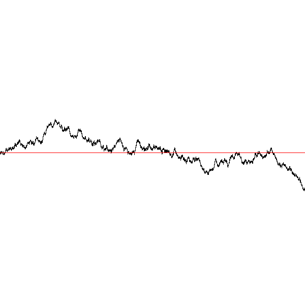
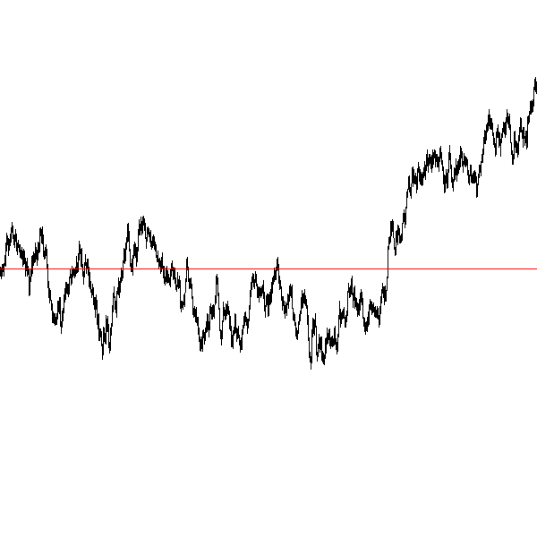
Even though we have a 50-50 chance of increasing or decreasing our chip count on every roll notice that we still go on long winning or long losing streaks.
Modify the random walk above so that whenever we have a positive chip count we plot a green pixel. For a negative chip count plot a red pixel.
Replace the line that plots a point with the condition:
1
2
3
4
if cash > 0:
win.set_at((i//scale, h//2-cash), color.green)
else:
win.set_at((i//scale, h//2-cash), color.red)
What color pixel gets plotted when cash equals 0? Does it matter? No, drawing the red line erases whatever pixel that would have been drawn at \(y\)-coordinate \(0\).
Modify the random walk so that whenever we hit a new high we mark the location by printing a small green circle (slightly bigger than a single pixel). Also, when we hit a new low, plot a red circle at the location.
The trick here is to use two variables, one to keep track of the current high, and the other to keep track of the current low. Call these high and low and should be initialized to the starting cash amount at the beginning. Whenever the cash variable exceeds high, set high to cash. Similarly when cash is less than low set low to cash.
1
2
3
4
5
6
if cash > high:
high = cash
pygame.draw.circle(win, color.green, (i//scale, h//2-cash), 2)
elif cash < low:
low = cash
pygame.draw.circle(win, color.red, (i//scale, h//2-cash), 2)
Here is an example run. Early in the simulation we generate lots of new highs and lows, and whenever we hit a new high or low we tend to generate several nearby, but these becaome rare as the simulation progresses. This was done with scale set to 100.
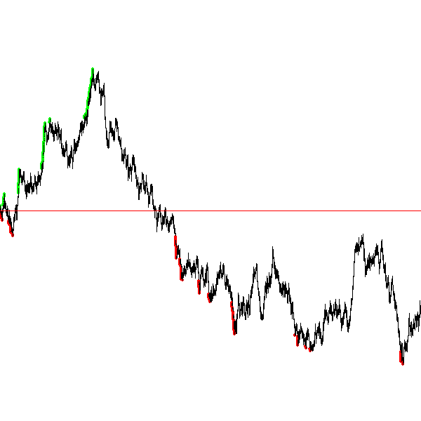
The Gambler’s Ruin is an example of a random walk. Random walks are useful for building models in many disciplines including economics.[18] and physics. In economics random walks are often used to model fluctuations in random processes such as the stock market. In physics, a random walk can model random motions such as Brownian Motion.
Random walks have a sophisticated and complex mathematical theory. However, notice how straightforward it is to do some simple programming experiments and learn something about random processes without having to understanding the mathematics.
The Gambler’s Ruin is an example of a _one dimensional random walk. One dimensional because there is only one random variable, the coin toss.
6.2. Brownian Motion
Brownian Motion is the random movement of particles suspended in a liquid or gas. Botanist Robert Brown discovered this while noticing the random movement of pollen particles on the surface of water. In this case, the particle can move randomly in either the \(x\) or \(y\) direction. In terms of a graphic display, the particle’s coordinate \((x,y)\) has eight possible neighboring locations that it can move to. Forgetting, for the time being, about a particle that is on an edge of the display.
In this case we will have two random variables, one in the \(x\) direction and one in the \(y\) direction. If (x,y) is the coordinate of the particle how can we make it move randomly to one of the eight neighbors? One way is to toss an eight sided die and update x and y accordingly. For example, if we assign each neighbor one of the random numbers from 0 to 7 with 0 corresponding to the top middle, then if we rolled a 0 then the particle’s new x coordinate would remain the same and its new y coordinate would be y - 1.
| Because we are using two random variables this Brownian Motion simulation is often referred to as a two dimensional random walk. It also goes by the rather uncomplimentary moniker The Drunkard’s Walk, referring to the rather haphazard way one who has imbibed too much alcohol meanders through the streets. |
1
2
3
4
5
6
7
8
9
10
11
12
13
14
15
16
17
18
19
20
21
dir = random.randrange(8)
if dir == 0: # top middle
y = y - 1
elif dir == 1: # top right
x = x + 1
y = y - 1
elif dir == 2: # right middle
x = x + 1
elif dir == 3: # lower right
x = x + 1
y = y + 1
elif dir == 4: # botton middle
y = y + 1
elif dir == 5: # bottom left
y = y + 1
x = x - 1
elif dir == 6: # left middle
x = x - 1
else: # top left
x = x - 1
y = y - 1
This block of code is the process we need to repeat over and over (when do we quit?, hold that thought). But first lets think about this code segment. Putting this in the loop body will make our loop a little unwieldy. Instead lets think of it in terms of a function move that takes a particle’s current x and y coordinate and returns its new x and y. Pictorially,
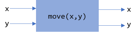
1
2
3
def move(x,y):
# insert if-elif above
return (x,y)
Calling the move function is the heart of our loop body. We can start a particle in the middle of the window (or at any random location for that matter) and let it run.
But when should the simulation stop? That is, what is the loop condition? We have several options. We could
-
run for a certain number of iterations, 10, 100, 10000, etc.
-
run until the particle moves off of the display
The first option is straightforward and just requires a counting variable. The second option is a little more interesting. How can we say, as a Python logical condition, while the particle is on the display?
Write a logical condition that is true if the particle at coordinate (x,y) is within the bounds of the display window. Assume that variable w and h refer to the width and height of the display.
Well … x must be between 0 and w (including 0, but excluding w) and
y must be between 0 and h (including 0, but excluding h):
(0 <= x and x < w) and (0 <= y and y < h)The parentheses are not strictly necessary but aid in clarity. Contrast this same expression without parentheses.
0 <= x and x < w and 0 <= y and y < hPython allows for a more concise way to describe inequalities. For example, in mathematical notation for the first inequality above, we would say \(0 \le x \lt w\). Python allows something similar and we can write 0 <= x < w. Most programming languages do not allow this more pithy notation, but Python does. So we could rewrite the logical expression as:
(0 <= x < w) and (0 <= y < h)6.2.1. The complete Brownian program
Putting this altogether we have …
1
2
3
4
5
6
7
8
9
10
11
12
13
14
15
16
17
18
19
20
21
22
23
24
25
26
27
28
29
30
31
32
33
34
35
36
37
38
39
40
41
42
43
44
45
46
47
48
import pygame, random, color
#
# move a particle with coordinates (x,y) to
# a new random location, one of its eight neighbors.
#
def move(x,y):
dir = random.randrange(8)
if dir == 0:
y = y - 1
elif dir == 1:
x = x + 1
y = y - 1
elif dir == 2:
x = x + 1
elif dir == 3:
x = x + 1
y = y + 1
elif dir == 4:
y = y + 1
elif dir == 5:
y = y + 1
x = x - 1
elif dir == 6:
x = x - 1
else:
x = x - 1
y = y - 1
return (x,y)
# main program
pygame.init()
win = pygame.display.set_mode((600,600))
w = win.get_width()
h = win.get_height()
x = w//2 (1)
y = h//2 (2)
win.fill(color.white)
while (0 <= x < w) and (0 <= y < h):
win.set_at((x,y), color.blue)
(x,y) = move(x,y)
pygame.display.update()
input("Hit enter")
| 1 | Start the particle in the middle of the x axis. |
| 2 | Start the particle in the middle of the y axis. |
Here is one sample run of the program
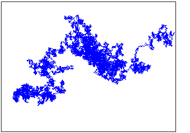
Add a second particle (use a different color) to the simulation. Stop the simulation when both particles have gone off the window.
Hints:-Add properties for a second particle. Don’t modify the move function or make a copy of the move function. Just reuse it by calling it again with the properties of the second particle. (That is the whole point of using functions). Finally modify the loop condition so the simulation terminates properly.
Like always, there are many solutions. Here is one.
1
2
3
4
5
6
7
8
9
10
11
12
13
14
15
16
17
18
19
20
21
22
23
24
25
26
import pygame, random, color
# same move function goes here.
# main program
pygame.init()
win = pygame.display.set_mode((600,600))
w = win.get_width()
h = win.get_height()
x1 = w//2 (1)
y1 = h//2
x2 = w//2 (2)
y2 = h//2
win.fill(color.white)
while (0 <= x1 < w) and (0 <= y1 < h) or \ (3)
(0 <= x2 < w) and (0 <= y2 < h):
win.set_at((x1,y1), color.blue)
win.set_at((x2,y2), color.green) (4)
(x1,y1) = move(x1,y1)
(x2,y2) = move(x2,y2) (5)
pygame.display.update()
input("Enter")
| 1 | Coordinates of the first particle. |
| 2 | Coordinates of the second particle. |
| 3 | Why logical or? |
| 4 | Don’t forget to draw the second particle. |
| 5 | Notice how we just call the move function a second time with different arguments? |
How hard is it to add a third particle? A fourth? As we progress we will learn more advanced techniques so we don’t have to keep defining new variables for each particle.
A two particle system might look like
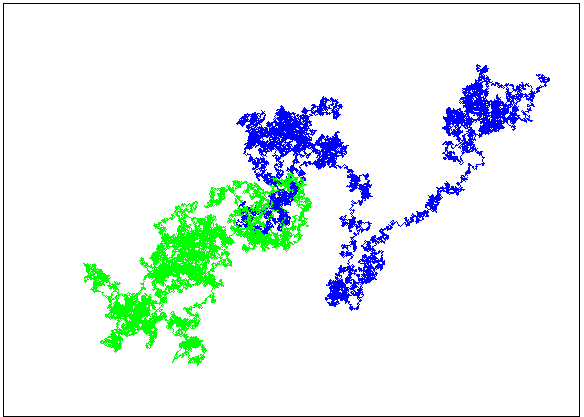
6.2.2. Improvement’s to the Brownian Program
That big if-statement in the move function is rather clunky and error prone. If you mistype a - or + sign then the particle goes off in a seemingly nonrandom direction. Notice that all we are doing is either subtracting 1 or adding 1 to the particle’s \(x\) and/or \(y\) coordinate. We could just generate a random integer in the range -1 to 1 and add that to the coordinate. We have to be careful to generate a different random integer for each coordinate.
A better and more concise move function.
1
2
3
4
5
6
7
8
9
def move(x,y):
delta_x = random.randrange(-1,2) (1) (2)
x = x + delta_x
delta_y = random.randrange(-1,2)
y = y + delta_y
return (x,y)
| 1 | Why 2 instead of 1 as the second argument to randrange? |
| 2 | The Greek letter \(\Delta\) (pronounced delta) is often used to represent a change in some quantity. In this case a change in the x coordinate. |
| Python (version 3) actually does allow Greek alphabetic letters in identifier names. |
Right now our particle simulation terminates when a particle hits the edge of the display. One modification would be to force the particle to stay within the bounds of the window. For example, when it hits an edge just make sure we don’t adjust the coordinate to go off the display.
Modify the Brownian particle simulation so that a particle stays within the bounds of the window as if the edges of the window were an impermeable wall.
The only thing you need to add is an if-statement that checks the bounds of the particle. An appropriate place to put this is the move function, since it is related to moving the particle.
1
2
3
4
5
6
7
8
9
10
# add this to the bottom of the move function.
if x >= w: (1) (2)
x = w - 1 (3)
elif x < 0: (4)
x = 0
if y >= h:
y = h - 1
elif y < 0:
y = 0
| 1 | Why >=? |
| 2 | Could we have also said x > w - 1 or even x == w? Yes to both. |
| 3 | Why w - 1? |
| 4 | Could we have also said x == -1? Yes. |
Another more interesting solution might be to pretend that the display wraps around on its edges. For example, if a particle goes off the right edge have it come in on the left edge, and vice-versa. If a particle goes off the top then it appears at the bottom.
An obvious way to do this is similar to the above check yourself solution and check if the particle has gone off an edge and reset its coordinate accordingly.
1
2
3
4
5
# wrap the x-coordinate around the x-axis.
if x >= w:
x = 0
elif x < 0:
x = w - 1 (1)
| 1 | Why w - 1 and not w? |
Modifying the \(y\)-coordinate is similar.
If we think of the display as a sheet of paper and curl the paper around on the x-axis then we curl it again around the y-axis we end up with the topological shape of a torus, or a donut.
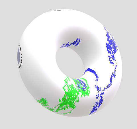
The concept of a variable wrapping around should be familiar. This is modular arithmetic. So rather than the if-statement above we can simply add or subtract 1 modulo the width or height of the window. In which case our move function becomes …
1
2
3
4
5
6
7
8
9
def move(x,y):
delta_x = random.randrange(-1,2)
x = (x + delta_x) % w
delta_y = random.randrange(-1,2)
y = (y + delta_y) % h
return (x,y)
Lets see what happens when the particle is on the right edge. Lets assume that the width of the window is 600 pixels (w is 600), x is 599. Lets further assume that delta_x is 1, then the new value of x is (599 + 1) % 600 or 0, which becomes the new value of x, effectively wrapping around to the left edge.
Lets look at the left edge. When the particle x is on the left edge then x is 0 and let delta_x be -1. Then (0 + -1) % 600 is -1 % 600 which is 599, effectively wrapping back to the right edge.
6.3. A Fractional Dimension Random Walk (or Fractal)
Imagine a hiker out for a hike got lost. Off in the distance the hiker sees three cell towers, call them \(t_0\), \(t_1\), and \(t_2\). The hiker picks a cell tower at random and heads off to it in a straight line. Halfway there the hiker changes their mind, and marks the spot with a rock (a thumb tack in the image below). The hiker then chooses another tower at random (maybe the same towser) and walks towards it, gets halfway there and has a change of heart. They once again mark the spot with a rock, and choose another cell tower. Continuing this process until, well, … forever. The image drawn by marking the rocks is an interesting sort of random walk.
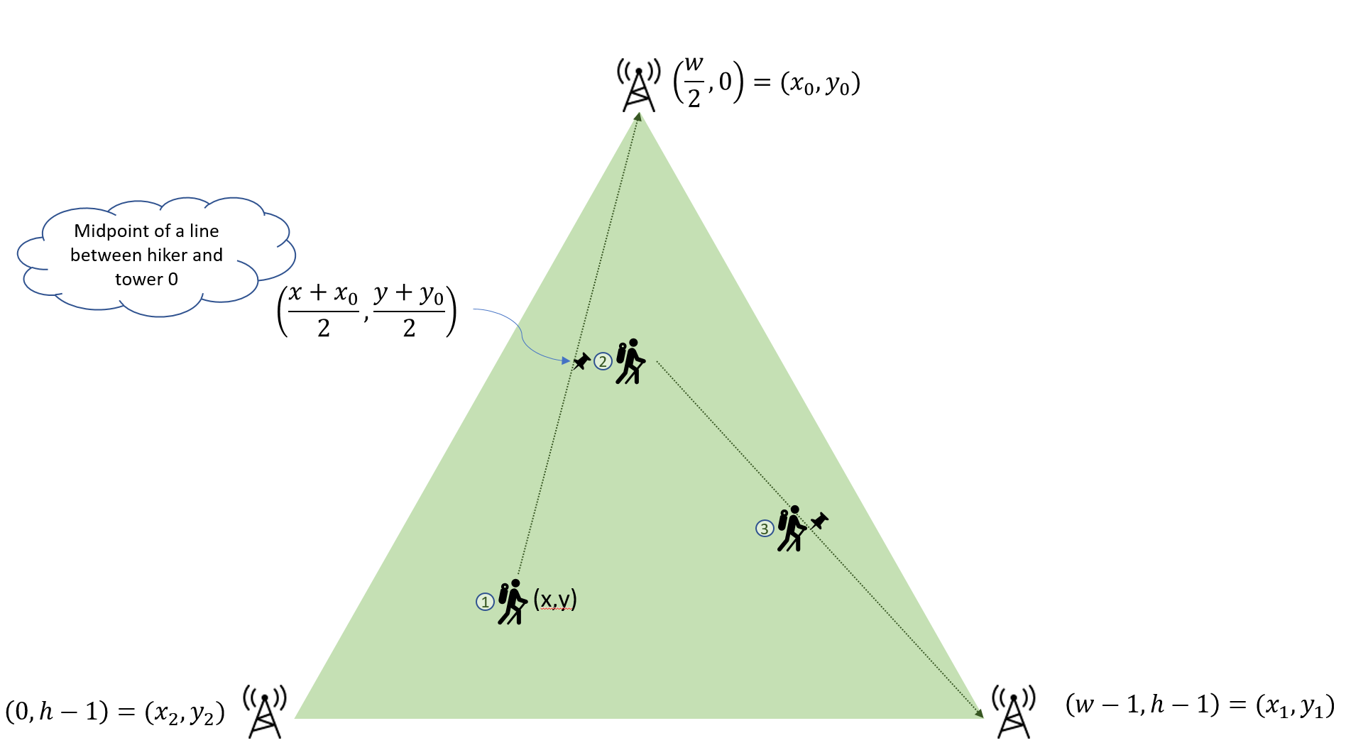
Let variables (x0,y0), (x1,y1), (x2,y2) be the coordinates of the towers, and
(x,y) be the coordinates of the hiker. Lets right down the process described in the paragraph above in pseudocode.
1) create a Pygame display window
2) Assign the coordinates of the towers to variables
3) Assign the hiker random coordinates anywhere within the display
4) Forever
   a) choose a tower at random
   b) compute the mid-point between the hiker and the chosen tower and
      update the hiker's coordinates with the midpoint.
c) plot a pixel at the hikers coordinate (similar to marking with a rock)| Before you start writing code make sure you understand the problem. One way to do this is to write out each step of the problem, not in real Python code, but in more informal text, what computer scientists call pseudocode. |
| The mid-point of a line between two points \((x_0,y_0)\) and \((x_1,y_1)\) is the average of the \(x\)-coordinates and the average of the \(y\)-coordinates, or \((\frac{x_0+x_1}{2}, \frac{y_0+y_1}{2})\). |
1
2
3
4
5
6
7
8
9
10
11
12
13
14
15
16
17
18
19
20
21
22
23
24
25
26
27
28
29
30
31
32
33
34
35
36
import pygame, random, color
side = 500
win = pygame.display.set_mode((side,side))
x0 = side // 2 # tower 0 coordinates (1)
y0 = 0
x1 = side - 1 # tower 1 coordinates
y1 = side - 1
x2 = 0 # tower 2 coordinates
y2 = side - 1
x = random.randrange(side) # hiker coordinates
y = random.randrange(side)
win.fill(color.white)
while True:
# choose a tower at random
t = random.randrange(3) (2)
# which tower is it?
if (t == 0):
x = (x + x0) // 2
y = (y + y0) // 2
elif (t == 1):
x = (x + x1) // 2
y = (y + y1) // 2
else:
x = (x + x2) // 2
y = (y + y2) // 2
win.set_at((x, y), color.blue)
pygame.display.update()
| 1 | Another way to write this is to use tuple assignment as (x0,y0) = (side//2, 0). |
| 2 | It is important that the random number is in the loop body. We need to get a new random tower every iteration. If this were before the loop then we would always be choosing the same tower. |
The shape rendered by the code is called Sierpinski’s Triangle.
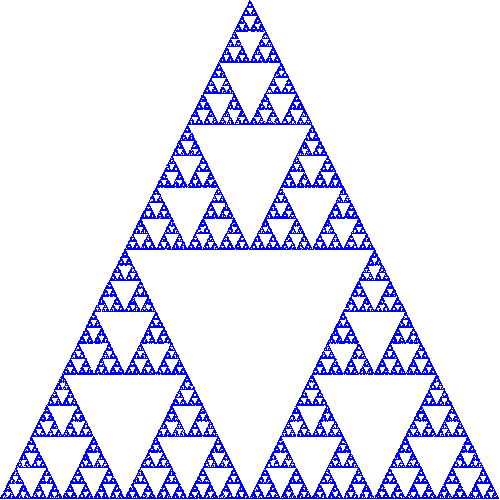
This process of choosing a random point within a shape and repeatedly choosing new points based on some criteria (e.g. the midpoint) is informally called the chaos game, named by the branch of mathematics called chaos theory.
The Gambler’s Ruin is an example of a one dimensional random walk, because the number of random variables is one, and the variable can take on any integer value. Brownian Motion is an example of a two dimensional random walk because there two random variable that can take on any integer value. Sierpinski’s Triangle is different. While there are two random variables, it is clear from the image that the variables can only take on a subset of the values that the two dimensional random walk can. It is some how less than a two dimensional random walk, but more than one dimensional. It is a fractional dimension random walk, or a fractal. The branch of Mathematics that studies fractals was made well know by the mathematician Benoit Mandlebrot in his book The Fractal Geometry of Nature.[19]
Add a second hiker to the Sierpinski Triangle program (the lost hiker example) and have it draw a different color pixel than the first hiker.
Rather than using a triangle use four cell towers, where each tower is placed in the middle of the window’s edge. For example, tower 0 is in the middle of the top edge at coordinate (side//2, 0), and so on. Additionally, when choosing a new random tower make sure not to choose the same tower twice in a row. Hint: Keep an extra variable prev that keeps track of the previous tower guessed . When choosing a new tower make sure that you keep guessing until it isn’t the same as prev.
6.4. The Monty Hall Problem
The Monty Hall Problem dates back to a game show on American television called Let’s Make a Deal, hosted by, of course, Monty Hall. In the game show a contestant is presented with three doors. Behind one of the doors is a new car and behind the remaining doors are goats.
The contestant chooses a door. Monty Hall then opens a door that has a goat behind it. So now there are two closed doors, the one the contestant chose and the one that Monty Hall did not open. The contestant is given the chance to switch doors. The Monty Hall Problem is whether the contestant should switch or not.
This problem caused quite a ruckus in the mathematics community when a reader of Marilyn Vos Savant’s weekly Parade column presented her with the problem.[21] Almost universally people thought the answer should be that it does not matter if the contestant switches because there are two unopened doors, so the odds are 50-50. Marilyn Vos Savant explained a different answer and the backlash from the mathematics community was harsh, patronizing, and really embarrassing for … the mathematicians. Marilyn Vos Savant was correct. This is easy for us to say now after-the-fact; hindsight is 20-20. This problem stumped some well known mathematicians, and to this day, many of us still fumble around when we try to explain it.
Probability is often counter-intuitive, we saw this with the Gambler’s Ruin, but once again we can explore the Monty Hall Problem by writing a rather simple program to simulate the Monty Hall Problem to explore the answer, without having to understand the mathematics. As we will see, even before we run the program, the answer will be evident.
Lets lay out the process of playing the game outlined above:
-
The contestant is presented with three doors, two with goats, and one with a new car. The goats and car are randomly assigned.
-
The contestant chooses a door to be revealed later.
-
The host shows a goat behind one of the other doors (not the contestant’s door).
-
The contestant is given the choice whether to switch to the other unopened door.
-
The contestant’s door is revealed.
We’ll tackle each of these in turn.
We can assign goats and a car to doors in any order. One thing we need to be careful about is that we do not assign more than one goat or car to the same door. Assume the doors are numbered 1, 2, and 3.
goat1 = random.randrange(1,4) (1)| 1 | Assign goat 1 to a random door. |
Now how about the second goat?
goat2 = random.randrange(1,4)This doesn’t quite work because we might accidentally get the same
random number as goat1. Here is another attempt.
goat2 = random.randrange(1,4)

if goat1 == goat2:
goat2 = random.randrange(1,4) (1)| 1 | Try again if we generated the same random door as goat1. |
This is a common mistake. Why is it incorrect? Well, while it is less likely, we can still get the same random number twice in a row. We need to keep trying as long as they are the same.
1
2
3
4
5
goat2 = random.randrange(1,4)
while goat1 == goat2:
goat2 = random.randrange(1,4) (1)
# What is true at this point after the loop terminates? (2)
| 1 | Keep trying as long as we keep getting the same random number as goat1. We know from the Gambler’s Ruin that we can sometimes get the same number several times in a row.
<2>that goat1 != goat2 |
We have now assigned the two goats to two different doors. We need to assign the car to the remaining door. We can do the same thing but we have to make sure to avoid the two goat doors.
1
2
3
car = random.randrange(1,4)
while car == goat1 or car == goat2:
car = random.randrange(1,4)
This is one way to do it.
Since there is only one door remaining for the car we should be able to calculate it without using a loop. Hint: Think of a simple expression involving the door numbers.
car = 6 - goat1 + goat2 (1)| 1 | Try it for various values of goat1 and goat2 |
In the second part of the game we need to have the contestant choose a door. We can simply ask them to input it from the keyboard.
choice = int(input("Choose a door: ")) (1)| 1 | We are assuming the user will type in either 1, 2, or 3. We don’t do any error checking, though error checking is an import part of writing reliable, robust computer programs. Indeed many computer security vulnerabilities come from software developers not properly validating input data causing programs to behave in unexpected and sometimes dangerous ways. |
So now we have four variables set up:
-
goat1the location of the first goat -
goat2the location of the second goat -
carthe location of the car -
choicethe door the contestant chose
In the third step of the game we reveal one of the two goats, being careful not to show what is behind the contestant’s door or where the car is. Lets set up two variables switch_door and show. The show variable will be the door we need to show and the variable switch_door will be the door the contestant will switch to if they decide they want to switch.
If the user chose the same door as goat1 then the door we will show is goat2. The door the user will switch to is (if these want to) is where the car is. The other cases are reasoned out the same way.
1
2
3
4
5
6
7
8
9
if choice == goat1: (1)
show = goat2
switch = car
elif choice == goat2: (2)
show = goat1
switch = car
else: (3)
show = goat1
switch = goat2
| 1 | If the contestant chose the same door as goat1 then we will show goat2 and if they choose to switch it will be to the car. |
| 2 | Similarly, if the contestant chose goat2 then we will show goat1 and if they choose to switch it will be to th car. |
| 3 | Finally, if the contestant chose the car then it doesn’t matter which goat to show. In this case we pick goat1 and we will show the goat2. |
We haven’t even finished the program yet and the solution to the Monty Hall Problem should be jumping out at you by examining the above if-statement. In two out of the three cases if the contestant switches doors they will switch to a car! Therefore, if they switch there is a two-thirds chance that they will win the car. They should definitely switch. Probability is often counterintuitive.
Finish the Monty Hall Program. Here are some sample runs of what the program might look like.
Choose a door: 1
There is a goat in door 3
Do you want to switch?(y/n): y
You won a goat!

Choose a door: 2
There is a goat in door 1
Do you want to switch?(y/n): y
You won a car!Below is just one version based on the code we’ve been developing.
1
2
3
4
5
6
7
8
9
10
11
12
13
14
15
16
17
18
19
20
21
22
23
24
25
26
27
28
29
30
31
32
33
34
35
36
37
38
39
40
41
42
43
44
45
46
47
48
49
import random
# place a goat behind door one.
goat1 = random.randrange(1,4)
# place the second goat, making sure
# that it is not the same door as the first goat.
goat2 = random.randrange(1,4)
while goat1 == goat2:
goat2 = random.randrange(1,4)
# how did the loop terminate?
# assign a car to the door that is not the
# same a goat 1 or goat 2
car = random.randrange(1,4)
while car == goat1 or car == goat2:
car = random.randrange(1,4)
# What is true?
# car != goat1 != goat2
# print(goat1,goat2,car)
choice = int(input("Choose a door: "))
# figure out how to show a goat
# to the contestant
if choice == goat1:
show = goat2
switch = car
elif choice == goat2:
show = goat1
switch = car
else:
show = goat1
switch = goat2
print("There is a goat in door", show)
switch_doors = input("Do you want to switch?(y/n): ")
if switch_doors == 'y' or switch_doors == 'Y':
choice = switch
# Did they win?
if choice == car:
print("You won a car!")
else:
print("You won a goat!")
What if we wanted to play the Monty Hall game many times to verify that the contestant should aways switch thereby winning the car two-thirds of the time? Running this version is a little cumbersome because it requires interaction with the keyboard. How can we automate playing the game thousands of times? When the user chooses a door, it is just a random choice. So we could have the computer choose a random door instead. Also, rather than ask whether the contestant wants to switch we hard code always switching. Finally, to play thousands of times we should probably wrap up our game in a function and put that function in a loop.
6.5. Exercises
Prime numbers play an important role in cryptography. A prime number is only divisible by
one and itself. If a number is not prime then it has a factor that is neither one or itself. For example,
\(16517\) has factors \(83\) and \(199\) because \(16517 = 83 \times 199\).
Write a program prime.py, that reads an integer from the user and prints whether the number is prime or not.
If we list all the natural numbers below 10 that are multiples of 3 or 5, we get 3, 5, 6 and 9. The sum of these multiples is 23. Write a program to print find and print the sum of all the multiples of 3 or 5 below 1000.[22]
Write a program that will read an integer and count and print the number of sevens that occur in the integer.
7. Case study: Particles and Collision
Let’s revisit modeling a particle moving in two dimensions at a constant velocity. We will use an image of particle (as a soccer ball) rather than a circle.

Assume that the particle is in an image file ball.png. We can load that image into
Pygame with pygame.image.load function. This function has one argument that is the name of the image file as a string constant. It returns a Pygame surface of the image.
1
ball = pygame.image.load("ball.png") (1)
| 1 | The variable ball is a Pygame surface. |
We have previously discussed Pygame surfaces noting that the Pygame display is a surface.
Here we are constructing a new kind of surface. The variable ball refers to a Pygame surface that is not the display surface, but a surface that represents an image and can be placed onto the display surface, like overlaying a smaller piece of paper on a larger piece of paper.
1
2
3
4
5
6
7
8
9
# Place a particle (an image of a soccer ball) on the display
import pygame, color
pygame.init()
side = 600
win = pygame.display.set_mode((side,side))
ball = pygame.image.load("ball.png").convert_alpha() (1)
win.fill(color.white)
win.blit(ball, (side//2, side//2)) (2)
pygame.display.update()
| 1 | The load function returns a surface. We immediately call the function convert_alpha on the surface so we don’t lose background transparency. |
| 2 | The function blit is used to place one surface on another. The term blit is an abbreviation for bit block transfer. |
Images are rectangular, even if they are an image of a circle. So in order for the image to appear like a circle the pixels that are outside of the ball are transparent. In graphics terminology we call this alpha transparency. The convert_alpha function ensures that when we load the image we don’t lose any of the transparency in the image pixels.
To animate a particle with a velocity we see that a velocity has two components, its direction on the \(x\)-axis and a direction on the \(y\)-axis. We often represent a velocity using two variables dx and dy. If dx were 1 then that means the particle would move to the right one pixel every time step. If dy were 1 then the particle would also move down one pixel every time step. The net effect would be that the particle would be moving down and to the right at a 45 degree angle.
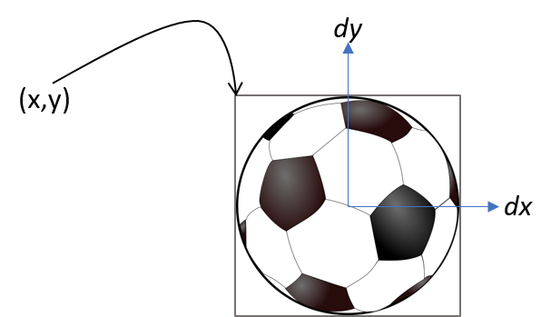
Unlike a Pygame circle, whose coordinate is measured from the center of the circle, the coordinates of an image in Pygame is the coordinate of the upper left corner of the image (remember, all images are rectangular).
All that is left to do is to update the particle’s coordinates by its velocity and do something sensible if it hits a wall. Let’s define a move function as we did in the Brownian Motion example. This move function will be a little more complicated because not only will the particle’s coordinates change (x and y), but if the particle hits a wall its direction will change, that is, the velocity dx or dy.
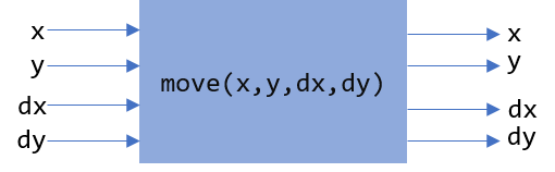
Here is an outline of the move function.
1
2
3
4
5
6
7
8
9
def move(x, y, dx, dy):
x = x + dx
y = y + dy
# detect if particle hits wall and modify
# dx or dy
return (x,y,dx,dy)
When a particle hits either the right or left wall its \(x\) velocity needs to reverse direction. Its \(y\) velocity will stay the same. For example, in the diagram below the particle is traveling from left to right and strikes the right wall.
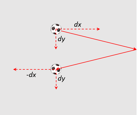
Here is the completed move function.
1
2
3
4
5
6
7
8
9
10
11
12
13
14
15
16
17
18
19
20
21
22
23
24
def move(x, y, dx, dy):
'''
x and y are the location of the particle
dx and dy is the velocity of the particle
return: new x, y, dx, and dy.
'''
x = x + dx
y = y + dy
if x < 0: # left wall
x = 0
dx = -dx
elif x + ball_w >= width: # right wall
x = width - ball_w
dx = -dx
if y < 0: # top wall
y = 0
dy = -dy
elif y + ball_h >= height: # bottom wall
y = height - ball_h
dy = -dy
return (x,y,dx,dy)
Now all that is left is to write the main program and call the move function.
We will start the particle off at the center of the display. For now, we’ll also initialize the velocity to very small numbers, less than 1. We will explain that later.
1
2
3
4
5
6
7
8
9
10
11
12
13
14
15
16
17
18
19
20
21
22
23
24
25
26
27
28
29
30
31
import pygame, color
pygame.init()
side = 600
win = pygame.display.set_mode((side,side))
width = win.get_width()
height = win.get_height()
ball = pygame.image.load("ball.png").convert_alpha()
# properties of the particle (ball)
ball_w = ball.get_width() # ball width
ball_h = ball.get_height() # ball height
ball_x = width//2 - ball_w//2 # center x coordinate
ball_y = height//2 - ball_h//2 # center y coordinate
ball_dx = .04 # x velocity
ball_dy = .01 # y velocity
while True:
# erase the old particle by redrawing the background
win.fill(color.lightgray)
# move the particle capturing its new position and possibly new velocity
(ball_x,ball_y,ball_dx,ball_dy) = \ (1)
move(ball_x, ball_y, ball_dx, ball_dy)
# draw the a particle on the screen
win.blit(ball, (ball_x, ball_y))
# update the display
pygame.display.update()
| 1 | Notice the line continuation character \. This is needed when a line is too long and you want to split it. |
The velocity variables dx and dy are set to be very small. .04 and .01. This goes against our intuition a little in that we are moving the particle four hundredths of a pixel in the \(x\) direction and one hundredth of a pixel in the \(y\) direction. Can we have fractions of a pixel? Well, no. But if we were to set these values to say 4 and 1, the loop executes so fast that the particle looks like it is just jumping around the screen and not moving fluidly. We could add a delay in the loop body using pygame.time.delay. Indeed we are going to do something similar but we want a more general solution for different speed computers; laptops vs desktops, macs vs windows, etc. We don’t want the ball to move across the screen in a shorter amount of time just because it is running on a faster computer.
7.1. Understanding the Frame Rate
One problem with the particle simulation above is that it will run faster or slower depending on the hardware it is running on. The animation runs as fast as the while loop can run. On slower computers the particle will move more slowly and more quickly on faster computers. Even if you have a faster computer that is doing a lots of other work the animation will slow down. One issue is that our velocity ball_dx and ball_dy are in pixels. But pixels per what? Velocity is always something like miles per hour or feet per second, or kilometers per hour. Our velocity does not have time associated with it. It is just, for example, .04 pixels per loop iteration. But how long does one loop iteration take to run?
A frame is one still image, a snapshot, of an animation. A standard frame rate for movies is 24 frames per second (fps). The movie The Hobbit: The Desolation of Smaug was filmed at 48 fps.
| A frame is one image in a sequence of images that is part of a video. The frame rate is the number of frames that are displayed per second of video. Common frame rates are 24, 30, 60. It was common for hand drawn cartoons to run at 15 fps. |
The particle simulation runs at one frame per loop iteration. This is enormously fast. On my laptop 1000 loop iterations takes about 1 second. That would amount to 1000 fps. The problem is that we do not know how long a loop iteration takes to execute. So we do not have a consistent frame rate.
Let’s instead define a velocity in terms of time as pixels per second. If our window is 600 pixels wide and we want the particle to travel across the window in two seconds then the \(x\) velocity would be 600 / 2.0 or 300 pixels per second. We should be more general and handle displays of various widths and heights. Assume width and height are the dimensions of the display we have …
1
2
ball_dx = width / 2 # travel across display in two seconds
ball_dy = height / 4 # four seconds to travel from top to bottom
We need to know how far the particle traveled in one loop iteration. This is where pygame’s Clock object is helpful. We can create a clock to measure time using …
clock = pygame.time.Clock()and we can call the object’s tick method that will return how many milliseconds have passed since the previous call to tick.
dt = clock.tick() (1)| 1 | let dt mean delta time or the change in time. In this case milliseconds. |
We can then compute how far the particle has traveled in both the \(x\) and \(y\) direction. If you all traveling at 55 MPH and 13 minutes has passed, then you have traveled \((13/60)55 = 14.67\) miles. The formula is the same for figuring out how many pixels we have traveled; though we need to convert milliseconds to seconds by dividing by 1000.
1
2
3
dt = clock.tick(60) / 1000.0 # in seconds
ball_x = ball_x + dt * ball_dx (1)
ball_y = ball_y + dt * ball_dy (2)
| 1 | The particle’s new \(x\)-coordinate is the old \(x\)-coordinate plus the time passed times the ball’s \(x\) velocity. This should make intuitive sense. |
| 2 | Similarly for the change in the \(y\) component. |
The logic for bouncing the particle off of the wall is exactly the same as before. We now have enough to rewrite our move function to account for the frame rate.
1
2
3
4
5
6
7
8
9
10
11
12
13
14
15
16
17
18
19
20
21
def move(x, y, dx, dy):
x = x + time_passed * dx
y = y + time_passed * dy
# bounce of the four walls (1)
if x < 0: # left
x = 0
dx = -dx
elif x + ball_w >= width: # right
x = width - ball_w
dx = -dx
if y < 0: # top
y = 0
dy = -dy
elif y + ball_h >= height: # bottom
y = height - ball_h
dy = -dy
return (x,y,dx,dy)
| 1 | This conditional is exactly like before. |
Piecing this all together we have …
1
2
3
4
5
6
7
8
9
10
11
12
13
14
15
16
17
18
19
20
21
22
23
24
25
26
27
28
import pygame, color
pygame.init()
side = 600
win = pygame.display.set_mode((side,side))
width = win.get_width()
height = win.get_height()
ball = pygame.image.load("ball.png").convert_alpha()
ball_w = ball.get_width()
ball_h = ball.get_height()
ball_x = width//2 - ball_w//2
ball_y = height//2 - ball_h//2
# particle velocity
ball_dx = width // 2 (1)
ball_dy = height // 4 (2)
# a clock object for handling the frame rate
clock = pygame.time.Clock()
while True:
time_passed = clock.tick(60) / 1000.0 (3)
win.fill(color.lightgray)
(ball_x,ball_y,ball_dx,ball_dy) = move(ball_x,ball_y,ball_dx,ball_dy)
win.blit(ball, (ball_x, ball_y))
pygame.display.update()
| 1 | move across \(x\) axis in two seconds |
| 2 | move down \(y\) axis in four seconds |
| 3 | The tick function can take an optional frame rate as an argument (in this case 60), which means Pygame will make sure that the loop does not go faster than 60 fps. |
Add a second particle to the simulation. Hint: you will need variables for the second particle’s position and velocity.
Create variables for the second particle’s position and velocity. Use different values than for the first particle to make it more interesting.
1
2
3
4
5
# this goes before loop
ball2_x = width // 4 - ball_w // 2
ball2_y = height // 4 - ball_h // 2
ball2_dx = width / 1.603 # across screen in 1.6 seconds (units are pixels/second)
ball2_dy = height / -3.237 # up screen in 3.2 seconds
Now modify the loop body to move the second particle. Remember to redraw the second particle.
1
2
3
4
5
6
7
8
9
10
11
while True:
win.fill(color.lightgray)
(ball1_x, ball1_y, ball1_dx, ball1_dy) =
move(ball1_x, ball1_y, ball1_dx, ball1_dy)
(ball2_x, ball2_y, ball2_dx, ball2_dy) =
move(ball2_x, ball2_y, ball2_dx, ball2_dy) (1)
win.blit(ball, (ball1_x, ball1_y))
win.blit(ball, (ball2_x, ball2_y)) (2)
pygame.display.update()
| 1 | Need to call move for the second particle.See how handy using a function is so we don’t have to cut-and-paste all of that code! |
| 2 | Draw the second particle. |
7.2. Collision Detection
How can we detect when the two particles collide? One way is to notice that if two particles overlap at all then the distance between the center of the two particles must be less than two times the radius of the particle (assuming the particles have the same radius).
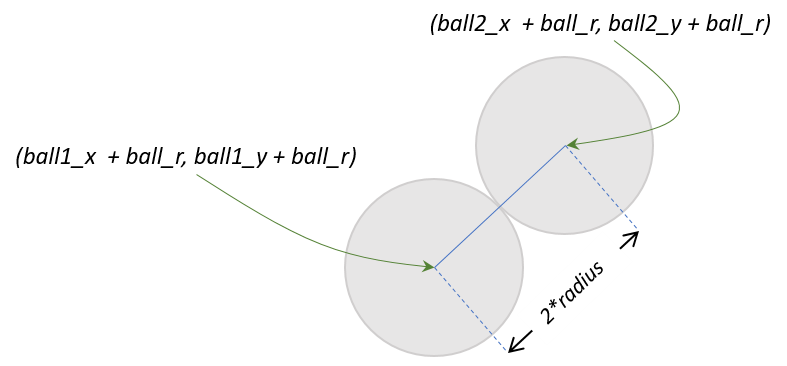
We can use the formula for the distance between two points to see if the center of the particles are less than the sum of the radius of each particle.
| Collision detection, detecting when two objects on a display collide, can be complicated. It is relatively straightforward in the case of two circles, but imagine more complex or irregular shapes. |
\(d=\sqrt{(x_2 - x_1)^2 + (y_2 - y_1)^2}\)
And we can write a nice function for:
1
2
3
# compute the distance between point (x1,y1) and (x2,y2)
def distance(x1,y1,x2,y2):
return math.sqrt((x1 - x2)**2 + (y1 - y2)**2)
But how should we handle the collision? In billiards, imagine the cue ball striking a stationary 8 ball dead on. If perfectly struck the cue ball will stop dead with all of its velocity transferring to the 8 ball. So the velocity of the cue ball was transferred to the 8 ball and the velocity of the 8 ball was transferred to the cue ball. That is, they swapped velocities.
To swap \(x\) velocities we need to introduce a temporary variable, tmp.
1
2
3
tmp = ball1_dx
ball1_dx = ball2_dx
ball2_dx = tmp
Write the code to swap the \(y\) velocities.
1
2
3
tmp = ball1_dy
ball1_dy = ball2_dy
ball2_dy = tmp
This is the classic way to express this in just about every programming language. Python’s tuple notation allows us to write this a little more succinctly. Two swap the value of two variables in Python you can use tuple assignment. For example, to swap the two variables a and b you can simply write …
(a,b) = (b,a)Notice that there is a tuple on the left hand side of =, the assignment operator. Up until now we have only ever had a single variable.
To wrap up collision detection we need to check if the particles are colliding, in the loop body we can write.
1
2
3
4
if distance(ball1_x + r, ball1_y + r,
ball2_x + r, ball2_y + r ) < 2 * r: (1)
(ball1_dx, ball2_dx) = (ball2_dx, ball1_dx) (2)
(ball1_dy, ball2_dy) = (ball2_dy, ball1_dy) (3)
| 1 | Assuming that r is the radius of the particle, it is just ball_w / 2. |
| 2 | Using tuple assignment here … |
| 3 | and here. |
| This way of handling a collision, simply swapping velocities, is overly simplistic and doesn’t take into account particles glancing of each other at angles. That involves a bit more math and trigonometry. |
Here is the entire program.
1
2
3
4
5
6
7
8
9
10
11
12
13
14
15
16
17
18
19
20
21
22
23
24
25
26
27
28
29
30
31
32
33
34
35
36
37
38
39
40
41
42
43
44
45
46
47
48
49
50
51
52
53
54
55
56
57
58
59
60
61
62
63
64
65
66
67
68
69
70
71
72
73
74
75
76
77
import pygame, color, math
pygame.init()
side = 600
win = pygame.display.set_mode((side,side))
width = win.get_width()
height = win.get_height()
ball = pygame.image.load("../images/ball.png").convert_alpha()
ball_w = ball.get_width()
ball_h = ball.get_height()
r = ball_w//2 # radius of the ball
# Properties of particle 1
ball1_x = width // 2 - ball_w // 2
ball1_y = height // 2 - ball_h // 2
ball1_dx = width / 2.02 # 2.02 seconds right
ball1_dy = height / 3.99 # 3.99 seconds down screen
# Properties of particle 2
ball2_x = width // 4 - ball_w // 2
ball2_y = height // 4 - ball_h // 2
ball2_dx = width / 1.1603 # 1.1603 seconds
ball2_dy = height / -2.237 # 2.237 seconds
# Function to compute the distance between two points.
def distance(x1,y1,x2,y2):
return math.sqrt((x1-x2)**2 + (y1-y2)**2)
# The move function. Moves a particle and bounces it
# off of the outer walls if needed.
def move(x, y, dx, dy):
dt = clock.tick(60) / 1000.0
x = x + (dt * dx)
y = y + (dt * dy)
if x < 0:
x = 0
dx = -dx
elif x + ball_w >= width:
x = width - ball_w
dx = -dx
if y < 0:
y = 0
dy = -dy
elif y +ball_h >= height:
y = height - ball_h
dy = -dy
return (x,y,dx,dy)
clock = pygame.time.Clock() # create a clock object
# The main outer loop.
while True:
win.fill(color.lightgray)
# move the particles
(ball1_x, ball1_y, ball1_dx, ball1_dy) =
move(ball1_x, ball1_y, ball1_dx, ball1_dy)
(ball2_x, ball2_y, ball2_dx, ball2_dy) =
move(ball2_x, ball2_y, ball2_dx, ball2_dy)
# check collision
if distance(ball1_x + r,
ball1_y + r,
ball2_x + r,
ball2_y + r ) < 2 * r:
(ball1_dx, ball2_dx) = (ball2_dx, ball1_dx)
(ball1_dy, ball2_dy) = (ball2_dy, ball1_dy)
win.blit(ball, (ball1_x, ball1_y))
win.blit(ball, (ball2_x, ball2_y))
pygame.display.update()
Add a third particle to the simulation and collision detection logic.
This gets to be a bit messy. We will have a better solution to handling multiple particles when we cover lists.
I left out the move and distance functions because they are exactly the same as previous.
1
2
3
4
5
6
7
8
9
10
11
12
13
14
15
16
17
18
19
20
21
22
23
24
25
26
27
28
29
30
31
32
33
34
35
36
37
38
39
40
41
42
43
44
45
46
47
48
49
50
51
52
53
54
55
56
57
58
59
60
61
62
63
64
65
66
67
68
69
70
71
import pygame, color, math
pygame.init()
side = 400
win = pygame.display.set_mode((side,side))
width = win.get_width()
height = win.get_height()
ball = pygame.image.load("ball.png").convert_alpha()
ball_w = ball.get_width()
ball_h = ball.get_height()
r = ball_w//2
# particle 1
ball1_x = width // 2 - ball_w // 2
ball1_y = height // 2 - ball_h // 2
ball1_dx = width / 2.02 # across screen in two seconds (units are pixels/second)
ball1_dy = height / 3.99 # down screen in four seconds
# particle 2
ball2_x = width // 4 - ball_w // 2
ball2_y = height // 4 - ball_h // 2
ball2_dx = width / 1.1603 # across screen in two seconds (units are pixels/second)
ball2_dy = height / -2.237 # down screen in four seconds
# particle 3
ball3_x = width - ball_w
ball3_y = height // 4 - ball_h // 2
ball3_dx = width / -0.8603 # across screen in two seconds (units are pixels/second)
ball3_dy = height / 1.237 # down screen in four seconds
clock = pygame.time.Clock()
while True:
win.fill(color.lightgray)
(ball1_x, ball1_y, ball1_dx, ball1_dy) =
move(ball1_x, ball1_y, ball1_dx, ball1_dy)
(ball2_x, ball2_y, ball2_dx, ball2_dy) =
move(ball2_x, ball2_y, ball2_dx, ball2_dy)
(ball3_x, ball3_y, ball3_dx, ball3_dy) =
move(ball3_x, ball3_y, ball3_dx, ball3_dy)
# check collisions
if distance(ball1_x + r, ball1_y + r,
ball2_x + r, ball2_y + r ) < 2 * r:
(ball1_dx, ball2_dx) = (ball2_dx, ball1_dx)
(ball1_dy, ball2_dy) = (ball2_dy, ball1_dy)
elif distance(ball1_x + r, ball1_y + r,
ball3_x + r, ball3_y + r ) < 2 * r:
(ball1_dx, ball3_dx) = (ball3_dx, ball1_dx)
(ball1_dy, ball3_dy) = (ball3_dy, ball1_dy)
elif distance(ball2_x + r, ball2_y + r,
ball3_x + r, ball3_y + r ) < 2 * r:
(ball2_dx, ball3_dx) = (ball3_dx, ball2_dx)
(ball2_dy, ball3_dy) = (ball3_dy, ball2_dy)
win.blit(ball, (ball1_x, ball1_y))
win.blit(ball, (ball2_x, ball2_y))
win.blit(ball, (ball3_x, ball3_y))
pygame.display.update()
for event in pygame.event.get():
if event.type == pygame.QUIT:
pygame.quit()
exit()
Adding a fourth and fifth particle is a lot of cutting-and-pasting. This should feel wrong. And it is. We’ll have a more general solution later on when we discuss lists where we can have as many particles as we want.
7.3. Exercises
Add an inner wall to the particle simulation that is centered within the display and has a width that is one tenth the width of the window and half of the height of the window. Have a particle bounce off of the left and right face of the wall. Don’t worry about the top and bottom. If it happens to hit the top it will look a little weird.
8. The for loop
Recall that a very common looping pattern is a counting loop that iterates an exact number of times. Recall the pattern …
1
2
3
4
i = 0
while i < n:
# loop body
i = i + 1
This loop body will execute exactly n times; as long as n is not modified in the loop body. Another way to write this in Python is using the for-loop.
1
2
for i in range(n):
# loop body
There are two new Python keywords for and in. There is also no explicit assignment statement incrementing i by one. There is also the use of this new function range(n) with an argument n. Technically range is not a function in Python but a range type which is used to generate an immutable sequence of integers. Something that is immutable cannot be changed. So range(n) generates a sequence of numbers from 0 up to but not including n.
The for-loop
1
2
for i in range(10):
print(i)
will print the integers 0 through 9, one per line. More generally, the for-loop has the syntax …
1
2
for var in some_sequence_type:
stmt
Where some_sequence_type represents a sequence of values, such as the sequence of integers generated by the range function. The variable var will take on each value in the sequence, and var can be used in the loop body, but var should never be modified in the loop body.
8.1. for loop examples
Here is an example for-loop that will sum the integers from 1 to 100.
1
2
3
total = 0
for i in range(101):
total = total + i
The range function can take an optional starting value. For example range(10,15) generates the sequence of integers 10, 11, 12, 13, 14 (it never includes the stop value, in this case 15).
1
2
3
4
5
# What is the output of the following code?
sum = 0
for i in range(3,8):
sum += i
print(sum)
25
Because 3+4+5+6+7 is 25.
1
2
3
4
5
# What is the output of the following code?
sum = 0
for i in range(8,3):
sum += i
print(sum)
0
Because the start value in the range function is greater-than-or-equal to the stop value,
the loop iterates exactly zero times.
The range function can also take an optional step value as the third argument. For example, range(10,15,2) generates the sequence of integers 10, 12, 14.
1
2
3
4
5
# What is the output of the following code?
sum = 0
for i in range(3,8,2):
sum += i
print(sum)
15
Because 3+5+7 is 15.
Step values can be negative. For example, range(8,3,-1) generates the sequence
8,7,6,5,4 (why does it not include 3? Because the range function never includes the
final stop value, in this case 3).
8.2. Nested for-loops
for-loops can be nested just like while loops. This is a pattern we will see frequently when we get to processing images in pygame. Consider the code fragment below:
1
2
3
for i in range(4):
for j in range(3):
print(i,'\t',j)
For each value of i in the outer for-loop j will take on values 0,1, and 2 in the inner for-loop. The output produced is:
0 	 0
0 	 1
0 	 2
1 	 0
1 	 1
1 	 2
2 	 0
2 	 1
2 	 2
3 	 0
3 	 1
3 	 2
This one is slightly more tricky, but one you will see again.
1
2
3
4
# What is the output of the following code?
for i in range(4):
for j in range(i,3):
print(i,'\t',j)
The way to think of this is that for each value i j will take on value from i
up to but not including 3.
0 	 0
0 	 1
0 	 2
1 	 1
1 	 2
2 	 2
8.3. Other kinds of for-loops
Later on we will see for-loops that don’t use integer ranges. That is, we will not always use the range function to generate a sequence for the for-loop. A string literal is also a sequence type, it is a sequence of characters. The code
1
2
3
name = "Tom Marvolo Riddle"
for ch in name:
print(ch)
will print each character in the string literal "Tom Marvolo Riddle" on a separate line. So a string is a sequence type. We will see several more sequence types, including strings, in later chapters.
8.4. Exercises
Conside a staircase of size \(n = 4\).
   #
  ##
 ###
####
The height and width are equal to \(n\). The image is drawn using # symbols and spaces. The last line does not have any spaces in it.
Complete the function staircase below. It should print a staircase as defined above. The input n is the size of the staircase (its width and height). Assume n is greater than 0.
Sample Input 0
6
Sample Output 0
     #
    ##
   ###
  ####
 #####
######
1
2
3
4
5
def staircase(n):
# fill in function body
# M a i n P r o g r a m
staircase(int(input('n: ')))
9. Event Handling
Up to this point the only way that the user has interacted with a program is to enter data from the console with the keyboard from a call to the input function. Lets now allow the user to interact with a running Pygame program using the mouse or the keyboard. For example, hitting the up and down arrows to move something on a pygame display or clicking somewhere on a pygame window.
| An event is a Pygame object that represents a user action such as pressing a key or moving the mouse. An event has data associated with it such as the kind of event, such as a mouse movement, mouse button press, or key press. Additional data depends on the event. For example, if the mouse was moved then the event also contains the current location of the mouse. If a key was pressed then the event contains data about which key. |
One event we can check for is to see if the user has clicked the X in the Pygame
window to kill the program. We can check for this event, named pygame.QUIT. Events can be generated quickly. Just moving your mouse across the Pygame display can generate hundreds of pygame.MOUSEMOTION events. Hence, events get stored in the event queue.
A queue is another name for a line. In the U.S. people might stand in a line to get a movie ticket, but in the U.K. people get in queue. An event queue is a Python object that holds events in the order they occur. When you are typing in your favorite word processor you want the characters to appear in the order they are typed. Anything else would be strange.
Here is a code snippet that checks for the QUIT event and stops the program if the user
has clicked on the X. The Pygame function pygame.event.get() retrieves the event queue (and the event queue is a sequence, so it can be used in a for-loop).
1
2
3
4
for event in pygame.event.get(): (1)
if event.type == pygame.QUIT: (2)
pygame.quit() (3)
exit() (4)
| 1 | For each event in the event queue |
| 2 | See if it is the QUIT event. If it is then … |
| 3 | stop Pygame (this is a new function) |
| 4 | exit out of the program |
We could place this code in the outer while loop of our particle simulation.
9.1. A Handy Utility Function
The above event processing code checks for a QUIT event while the program is executing. It does not otherwise cause the program to stop or wait. Recall how we were using the input() function to cause a Pygame program to actually pause so the display didn’t just disappear when the program terminated. Lets modify the above event processing code and write a function wait_for_quit() that causes the program to actually stop and wait until the user closes the window. We can do this just by looping until the user closes the window.
util.py1
2
3
4
5
6
7
8
def wait_for_quit():
while True:
for event in pygame.event.get(): (1)
if event.type == pygame.QUIT:
pygame.quit()
exit() (2)
pygame.time.wait(100) (3)
| 1 | Same event code as before. |
| 2 | wait_for_quit never returns, it just kills the program right here. |
| 3 | While this line not absolutely necessary, forcing a delay keeps the while loop from spinning at maximum speed and hogging the CPU thereby allowing other programs that might be running to utilize the CPU. Actions like this also keep your CPU cooler, and use less battery on your laptop. |
Function pygame.time.wait waits for a number of milliseconds. It is similar to pygame.time.delay except that pygame.time.wait relinquishes the CPU so that other programs may run whereas pygame.time.delay continues to use the processor during the delay.
|
Function wait_for_quit assumes that if the user closes the window they want the program to terminate as well. Function wait_for_quit() is so useful that we might consider putting it in a separate file util.py so we can import it in other Pygame programs.
Write a function wait_for_click() that pauses the program until the user clicks
somewhere in the Pygame display. This function should behave a little differently than wait_for_quit() in that the program should not exit, but just continue.
1
2
3
4
5
6
7
def wait_for_click():
done = False (1)
while not done: (2)
for e in pygame.event.get(): (3)
if e.type == pygame.MOUSEBUTTONDOWN: (4)
done = True (5)
pygame.time.wait(100) (6)
| 1 | Local variable used to control the while loop. |
| 2 | This loop does not terminate until the user has clicked in the Pygame display. |
| 3 | Standard code to get events in event queue. |
| 4 | Check for the MOUSEBUTTONDOWN event. This will check for either the left or right mouse button and even clicking the scrolling wheel on the mouse. |
| 5 | Setting done to True will cause the while-loop to terminate. |
| 6 | Again, this is to be user friendly and let other programs run and not chew up CPU (or battery). |
Function wait_for_click does actually return (unlike wait_for_quit). It also does not return a value (OK, it returns the special value None). We should also put wait_for_click in util.py.
9.2. Pong
One of the first successful video games was Pong. By now Pong is considered a classic, almost the hello world of computer games. Lets add a paddle to our particle simulation and bounce the particle off the paddle. First we will need a graphic for the paddle.

Next we need to set up some properties of the paddle and blit it to the display inside of the outer while. We’ll offset the paddle a little padding on the left and start it in the middle of the \(y\) axis of the display.
1
2
3
4
5
6
7
# properties of the paddle
paddle = pygame.image.load("paddle.png")
paddle_w = paddle.get_width()
paddle_h = paddle.get_height()
paddle_x = 10
paddle_y = height // 2 - paddle_h // 2
paddle_dy = 8
and add the following line right after we blit the ball in the outer while loop. (Okay, so we are playing pong with a soccer ball).
win.blit(paddle, (paddle_x, paddle_y))We need to figure out how to make the paddle responsive to the up and down arrow on the keyboard. The KEYDOWN event means that some key on the keyboard is being pressed. We can look at some data associated with the event to determine which key it is. We can
check to see if event.key is K_UP or K_DOWN, the constants for the up and down arrow keys and add or subtract to paddle_y as appropriate.
Our code to process events is a little more complicated.
1
2
3
4
5
6
7
8
9
for event in pygame.event.get():
if event.type == pygame.QUIT:
pygame.quit()
exit()
elif event.type == pygame.KEYDOWN: (1)
if event.key == pygame.K_UP: (2)
paddle_y = paddle_y - paddle_dy
elif event.key == pygame.K_DOWN: (3)
paddle_y = paddle_y + paddle_dy
| 1 | Do we have a key press event? |
| 2 | If so, then is it the up-arrow … |
| 3 | or the down-arrow key? |
When you add this to the outer while loop you will notice that you need to keep hitting the up or down arrow key just to move the paddle one pixel. That is because when you press the down arrow key you generate only one event. What we would like to have happen is that when we press the key we continue to generate KEYDOWN events at a regular interval as long as it stays pressed. We can do this at the start of the program using the Pygame function:
pygame.key.set_repeat(initial,interval)What this says is to generate an initial event after initial milliseconds and then at regular intervals of interval milliseconds as the key is pressed. Reasonable values for
initial and interval are 1 millisecond.
pygame.key.set_repeat(1,1)Moving the paddle one pixel at a time is still slow, so we’ll set up another variable paddle_dy to move it eight pixels every event.
In order to make this a complete Pong game we need some way to lose. In Pong this is by not hitting the ball and having go off the left edge. IN the move function we need to remove the code that bounces the particle off of the left wall. And in the outer while loop we can simply check the \(x\) coordinate of the ball and exit the program much like we did for the QUIT event.
Modify the move function so the particle does not bounce off of the left wall.
Simply delete the part of the condition where we check if \(x\) is less than 0. The new move function is below.
1
2
3
4
5
6
7
8
9
10
11
12
13
14
15
16
17
18
19
20
21
def move(x, y, dx, dy):
dt = clock.tick(60) / 1000.0 # time elapsed since last frame
x = x + dt * ball_dx # new x and y coordinates
y = y + dt * ball_dy
# code to bounce off of left wall was deleted here.
if x + ball_w >= width: # right wall
x = width - ball_w
dx = -dx
if y < 0: # top wall
y = 0
dy = -dy
elif y + ball_h >= height: # bottom wall
y = height - ball_h
dy = -dy
return (x,y,dx,dy)
Modify the outer while loop so that the game ends (rather abruptly) when the ball
goes off the left hand side of the window.
In the move function to check to see if the player lost we could add the following
code to the outer while loop.
1
2
3
4
# check to see if we lost.
if ball_x < 0:
pygame.quit()
exit()
Here is the entire outer while loop including our event code to check for the
QUIT event and the paddle movement.
1
2
3
4
5
6
7
8
9
10
11
12
13
14
15
16
17
18
19
20
21
22
23
24
25
26
27
28
pygame.key.set_repeat(1,1)
while True:
win.fill(color.lightgray)
(ball_x,ball_y,ball_dx,ball_dy) = \
move(ball_x,ball_y,ball_dx,ball_dy)
# check to see if we lost.
if ball_x < 0:
pygame.quit()
exit()
# handle events
for event in pygame.event.get(): (1)
if event.type == pygame.QUIT:
pygame.quit()
exit()
elif event.type == pygame.KEYDOWN:
if event.key == pygame.K_UP:
paddle_y = paddle_y - paddle_dy
elif event.key == pygame.K_DOWN:
paddle_y = paddle_y + paddle_dy
win.blit(ball, (ball_x, ball_y))
win.blit(paddle, (paddle_x, paddle_y))
pygame.display.update()
| 1 | This is the same as the event processing for loop we just covered above. |
The outer loop, in our case the while loop (throttled by the frame rate) is often called the game loop.
|
We also need to bounce the ball off of the paddle. To do this lets make sure we understand the various coordinates and widths and heights.
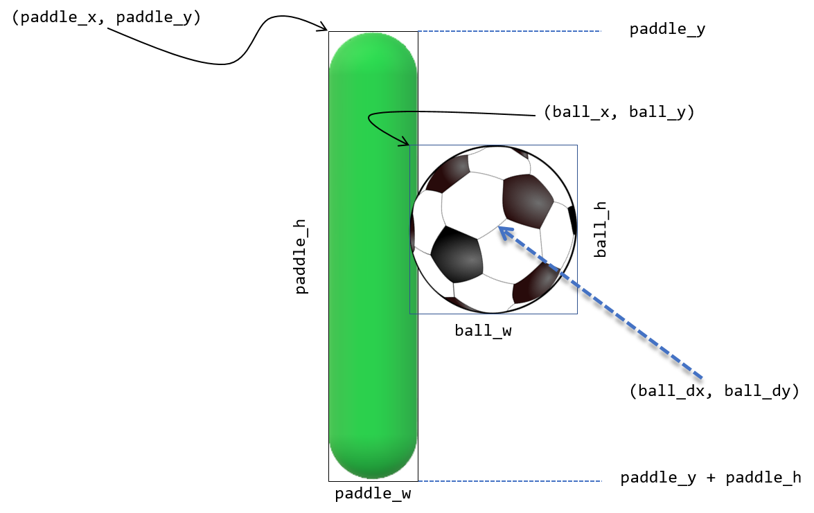
With the paddle on the left hand side of the display, the ball is always coming in from the right. One common mistake is to check if the \(x\) coordinate of the right side of the paddle (paddle_x + paddle_w) is equal to the left edge of the ball, ball_x.
1
2
if paddle_x + paddle_w == ball_x:
dx = -dx
But remember that the particle travels a certain distance each frame and the left edge of the ball will most likely overlap the right edge of the paddle and rarely be equal. We should check if the left edge of the ball is less than or equal to the right edge of the paddle.
1
2
if ball_x <= paddle_x + paddle_w:
dx = -dx
That’s closer. But this is true even if the ball goes off the left edge of the display. Now we need to check if the ball is within the \(y\) coordinates of the paddle.
1
2
3
if x <= paddle_x + paddle_w and \
paddle_y <= ball_y <= paddle_y + paddle_h: (1)
dx = -dx
| 1 | Using Python’s more mathematical notation for inequality \(x \le y \le z\) |
It probably makes sense for this to go in the move function for the ball to keep the body of the main loop less cluttered.
Modify the move function so that it properly checks to see if the ball bounces off of the paddle.
def move(x, y, dx, dy):

    dt = clock.tick(60) / 1000.0

    x += dt * ball_dx
    y += dt * ball_dy

    if x + ball_w >= width:     # right wall
        x = width - ball_w
        dx = -dx

    if y < 0:                   #top wall
        y = 0
        dy = -dy
    elif y + ball_h >= height:  # bottom wall
        y = height - ball_h
        dy = -dy

    # check if particle hits paddle.          (1)
    if x <= paddle_x + paddle_w and \         (2)
       paddle_y <= y <= paddle_y + paddle_h:
        dx = -dx

return (x,y,dx,dy)| 1 | This if-statement is the only modification to the move function. |
| 2 | We are using the parameters x and y and not ball_x and ball_y. Why? See the next check yourself. |
Add a second ball to the pong game. Lose when both balls have gone off the screen.
TBD
# TBD10. Image Processing
One important and common application in computer science is image processing. Computer vision, facial recognition, medical imaging (MRIs, x-rays, CT scans) are all part of image processing. Your smartphone has image processing software; the camera provides a software zoom, and the fingerprint sensor on the device has image processing software for fingerprint matching. Web browsers resize images, and software such as Photoshop is used to do some amazing effects with images.
From what we have learned so far in our explorations in programming, images are composed of pixels and a pixel is an RGB triple, three integers between 0 and 255. There is also a fourth integer that represents the alpha transparency of the pixel. An alpha value of 255 is a fully opaque pixel (what we have been using all along) and an alpha value of 0 is a fully transparent pixel. Alpha transparency is used to overlay pictures on top of each other, what we call compositing. We wont be using alpha transparency much, but we need to know it is there and that RGB color values really contain a fourth integer component. We should more properly call this the RGBA color scheme.
If an image is really just a bunch of integer values it means we can modify the pixel values in some way to come up with a new image. For example, what if we were to decrease each RGBA component of every pixel by 30%? Theoretically this should make the image darker.
To do this we need a systematic way to go through every pixel in the image so we don’t miss any. We can go through the image row-by-row or column-by-column. We can proceed either top to bottom, bottom to top, left to right, or right to left. Probably the most common way to process an image is row-by-row and top-to-bottom.
| An image is just a rectangular table of pixels, where each pixel is four integers. |
10.1. Interlude - processing rectangular data
Processing a rectangular table of numbers is common in computer science. We have a systematic way in which we can go through each number using two nested for loops. For example, lets say we wanted to produce the following 9 X 9 multiplication table on the console:
1	2	3	4	5	6	7	8	9
2	4	6	8	10	12	14	16	18
3	6	9	12	15	18	21	24	27
4	8	12	16	20	24	28	32	36
5	10	15	20	25	30	35	40	45
6	12	18	24	30	36	42	48	54
7	14	21	28	35	42	49	56	63
8	16	24	32	40	48	56	64	72
9	18	27	36	45	54	63	72	81
1
2
3
4
for i in range(1,10): (1)
for j in range(1,10): (2)
print(i * j, "\t", end="") (3)
print() (4)
| 1 | We call this the outer for-loop. It constructs the rows in the table. |
| 2 | We call this the inner for-loop. It is responsible for construction a single row. |
| 3 | Recall that the character \t represents the tab character. The third argument end="" is what we call a named parameter in Python. The print function takes an optional argument whose corresponding parameter name is end. The end parameter specifies how we should handle the end of line. In this case we don’t want the print statement to print the end-of-line character \n, so we suppress it with end="". |
| 4 | This starts a new line. |
| A matrix is a rectangular table of numbers. The branch of mathematics that deals with matrices is called linear algebra. |
Rewrite the two nested for-loops above using two nested while loops.
1
2
3
4
5
6
7
8
i = 1
while i < 10:
j = 1
while j < 10:
print(i * j, "\t", end="")
j = j + 1
print()
i = i + 1
10.2. Darken an Image
To darken an image we need to decrease the RGB value of each pixel by a certain amount, say 10%. In pseudocode we need something like …
for each row r in the image
   for each column c in row r
      get the RGBA components of pixel (c,r)
	  reduce each component by 10%
	  reset the pixel at (c,r) with the new RGBA values
A new Pygame function will assist us, surface.get_at( (x,y) ) returns the RGBA tuple at column x and row y. For example, if win was our surface, we could get the pixel in the upper left corner of the image with …
(r,g,b,a) = win.get_at((0,0)) (1)| 1 | To be more precise recall that functions like get_at are methods because they are called using an object. |
The Pygame function surface.set_at( (x,y), RGBA) modifies the pixel at coordinate (x,y) to be the color specified by RGBA (you can leave off the alpha transparency value, and just specify the RGB colors and the transparency will default to opaque). For example, to set the upper left corner pixel black …
win.set_at((0,0), (0,0,0)) (1)| 1 | The set_at function does not return a value. Recall that functions that do not return a value really return the special value None. |
Here’s a program that darkens the image below by 30%. We will review it line by line.
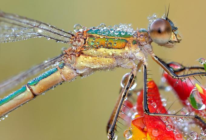
https://500px.com/martinamm accessed 7/27/2017, found at reddit link 1
2
3
4
5
6
7
8
9
10
11
12
13
14
15
16
17
18
import pygame, util
pygame.init()
image = pygame.image.load("bug.jpg") (1)
win = pygame.display.set_mode((image.get_width(), image.get_height())) (2)
image = image.convert_alpha() (3)
for y in range(image.get_height()): (4)
for x in range(image.get_width()): (5)
(r,g,b,a) = image.get_at((x,y)) (6)
r = r * .7 (7)
g = g * .7
b = b * .7
image.set_at((x,y), (r,g,b)) (8)
win.blit(image, (0,0)) (9)
pygame.display.update()
util.wait_for_click() (10)
| 1 | Load the image before we construct the display so we know how large to make the display. |
| 2 | Construct a display surface that is the same size as the image. |
| 3 | Call the convert_alpha() method after we load the image on line 4 and construct the display on line 5. This is because the the convert_alpha function is making the format of the image compatible with the format of the display. |
| 4 | For each row of pixels y. |
| 5 | For each pixel x ub row y. |
| 6 | Get the pixel value as the four components (r,g,b,a). |
| 7 | Decreasing a value by 30% is the same as multiplying it by .7. |
| 8 | We need to put the modified pixel values back in the image. |
| 9 | blit the modified image back in to the display. |
| 10 | Recall that the wait_for_click() function was defined in the section on event handling. |
And here is the result of darkening the image of the bug.
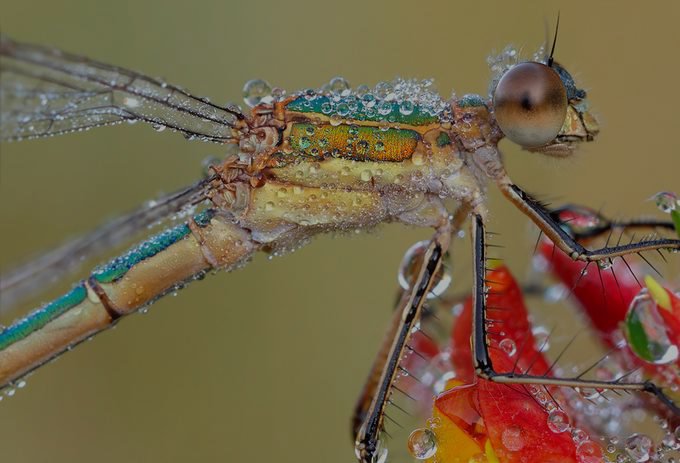
10.3. Converting an image to Grayscale (and more)
The code for darkening an image gives us a useful template for performing a variety of image processing examples. The pixels in a grayscale image (i.e., black-and-white) are always a shade of gray. Recall that in a gray pixel the RGB values are all equal.
Lets say in our color image we had a pixel that was a very dark color such as (93,15,13),
a dark maroon. We would expect the corresponding grayscale pixel to be dark as well, a dark gray. Conversely, we would expect a bright color such as yellow (255,255,0) to be a light gray. One technique is to average the pixels of the color and use the average of the three color components. For example dark maroon would get converted to
\((93 + 15 + 13)/3 = 40.3\), or the dark gray (40,40,40). Yellow would get converted
to \((255 + 255 + 0)/3 = 170\), or the light gray (170,170,170). We can almost reuse the entire program for darkening an image. Just change the inner loop body to …
1
2
3
(r,g,b,a) = image.get_at((x,y))
gray = (r+g+b)//3
image.set_at((x,y), (gray,gray,gray))
The result is …

What is cool with digital images is that we can do whatever we want to the pixel values. The term photographic negative comes from the era a film photography and how chemicals were used to develop film where colors are negated, white becomes black, black becomes white. For colors, the photographic negative of a pixel means to subtract each color component from 255.

Compute and display the photographic negative of the bug.
Just change the inner loop body to …
(r,g,b,a) = image.get_at((x,y))
image.set_at((x,y), (255 - r, 255 - g, 255 - b))
The result is pretty cool looking.
The possibilities are endless. What hapens if we switch the color components around? For example, for every pixel \((r,g,b)\) change it to \((g,b,r)\)? Sometimes the effects are surprising and beautiful.
(r,g,b,a) = image.get_at((x,y))
image.set_at((x,y), (g,b,r))
10.4. Scaling an Image
A common image processing operation is to resize an image so that it is larger or smaller. Lets think of this operation as a function that takes an image to resize along with the new width and new height of the resulting image.
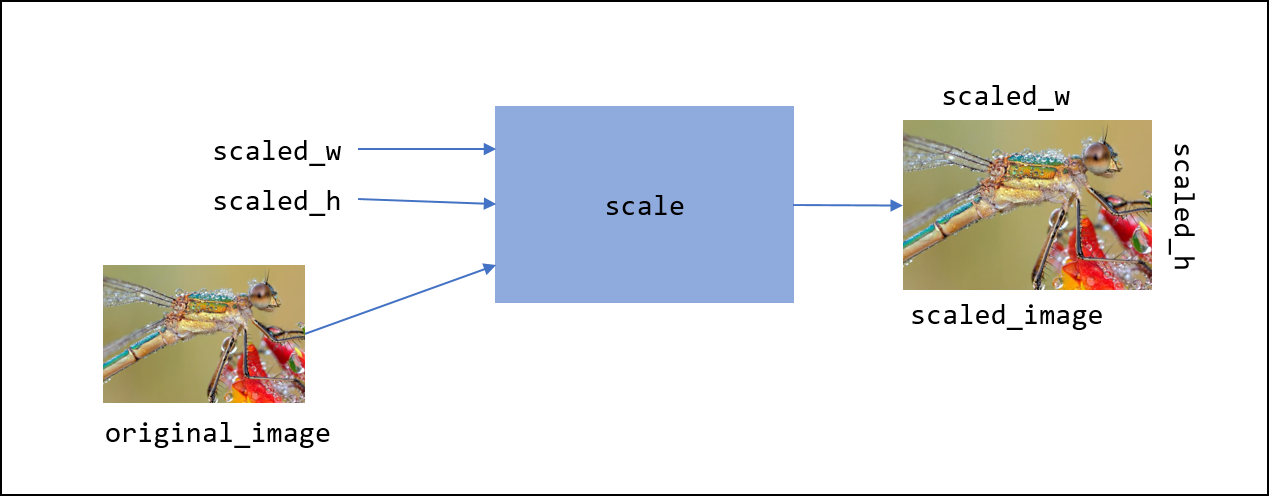
Until now we have had two ways to create a surface; the first is to use the pygame.display.set_mode function to create the special display surface. The second way was to use the pygame.image.load function to create a surface for an image. But our scale function will need to create an initially blank surface of an arbitrary width and height.
The Pygame following line
surf = pygame.Surface((w,h))creates a new empty surface surf with width w and height h and assigns it to the variable surf.
Lets assume we have an image we want to scale and it is in a surface image. Furthermore assume we have an empty surface surf that will be the new scaled image. We have to go through every pixel in surf and find a pixel in image to copy in to surf.
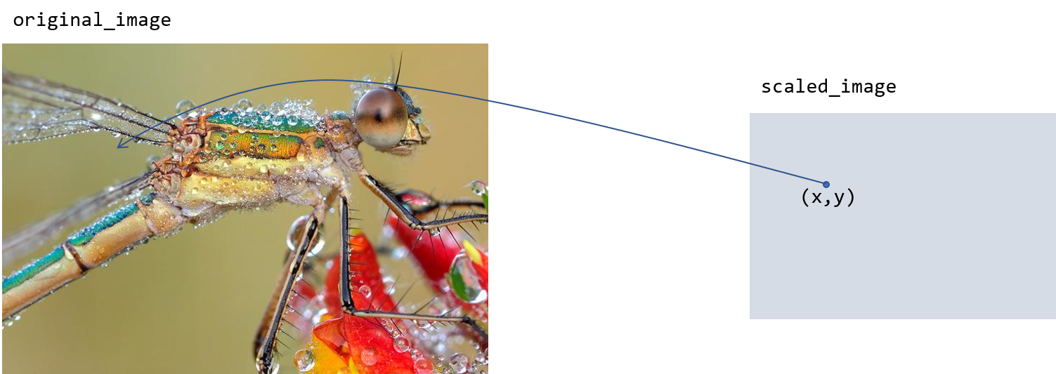
Lets say the orginal image was 600 pixels wide and the scaled image is 300 pixels wide. The \(x\) coordinate 10 in the scaled image should correspond to \(x\) coordinate 20 in the original image because the ratio of the widths in the original image to the scaled image is 2-to-1.
In general if the width of the original image is \(w\) and the width of the scaled image is \(w'\) then an \(x\) coordinate in the scaled image will correspond to the \(x\) coordinate \(xw/w'\) in the original image. The reasoning is the same for the \(y\) coordinate.
Here is the function scale.
1
2
3
4
5
6
7
8
9
10
11
12
13
14
def scale(original, scaled_w, scaled_h):
scaled = pygame.Surface((scaled_w, scaled_h)) (1)
w_ratio = original.get_width() / scaled_w (2)
h_ratio = original.get_height() / scaled_h (3)
for row in range(scaled_h): (4)
for col in range(scaled_w):
x = int(col * w_ratio) (5)
y = int(row * h_ratio)
(r,g,b,_) = original.get_at((x,y)) (6)
scaled.set_at((col,row), (r,g,b)) (7)
return scaled (8)
| 1 | Create the new empty surface that will contain our scaled image. |
| 2 | Compute the ratio of the original image’s width to the new scaled image’s width. |
| 3 | Compute the ratio of the original image’s height to the new scaled image’s height. |
| 4 | For every pixel in the scaled image … |
| 5 | Compute the \(x\) and \(y\) coordinates of the pixel we need to grab in the original image. |
| 6 | Get the pixel in the original image. |
| 7 | And copy it to the new scaled image. |
| 8 | Don’t forget this is a function that returns a new image. |
Notice that we use floating-point division on lines 4-5. This is because we might be shrinking an image by a non-integral amount. For example, to shrink an image from 200 X 200 pixels to 150 X 150 then w_ratio and h_ratio need to be 1.33 and not 1. When enlarging an image from 150 X 150 to 200 X 200 then w_ratio and h_ratio need to be 0.75 and not 0. On lines 9-10 we need to convert back to integer coordinates.
|
10.4.1. Shrinking an image
If we are shrinking an image then we only pick out a subset of the pixels in the original image. For example, if the original image was 400 X 400 and we are shrinking it to 200 X 200. The scaling ratios w_ratio and h_ratio are both 2. Pixel (0,0) in the scaled image maps to pixel (0,0) in the original image. But pixel (1,0) in the scaled image maps to pixel (2,0) in the original image. We skipped over pixel (1,0).
Use the scale function to shrink an image 1/3 of its original height and width. Display the original image and center the smaller image in the original.
1
2
3
4
5
6
7
8
9
10
11
12
13
14
15
16
17
18
19
20
21
22
import pygame, util
pygame.init()
image = pygame.image.load("bug.jpg")
win = pygame.display.set_mode((image.get_width(),
image.get_height())) (1)
image = image.convert_alpha() (2)
scaled_image = scale(image, image.get_width()//3,
image.get_height()//3) (3)
win.blit(image, (0,0)) (4)
tmp_x = win.get_width()//2 - scaled_image.get_width()//2 (5)
tmp_y = win.get_height()//2 - scaled_image.get_height()//2
win.blit(scaled_image, (tmp_x, tmp_y)) (6)
pygame.display.update()
util.wait_for_click()
| 1 | Create a display the size of the original image. |
| 2 | Always a good idea, but not always necessary. |
| 3 | Scale the original image. |
| 4 | Blit the original image on to the display. |
| 5 | Calculate the coordinates where scaled_image will be blitted. |
| 6 | Blit the scaled image. |
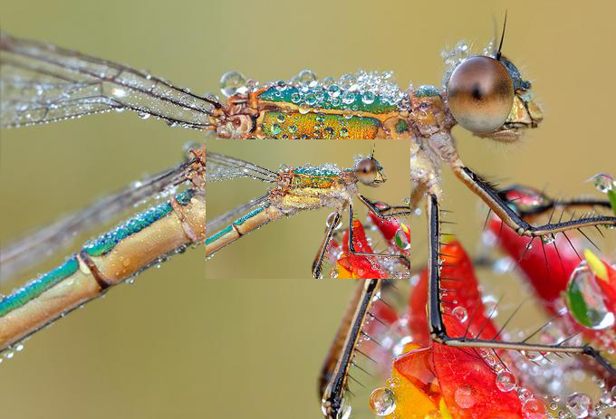
Notice how we scaled the width and height of the image by the same proportion. That is, we kept the aspect ratio of the image the same.
| The aspect ratio of an image is the ratio of an image’s width divided by its height. |
We didn’t have to keep the aspect ratio the same. The scale function will elongate, or stretch, an image along its horizontal or vertical axis.
10.4.2. Enlarging an image
Does our scale function work if we are trying to enlarge an image? Lets reverse the scenario and enlarge a 200 X 200 image to 400 X 400. In this case the scaling ratios w_ratio and h_ratio are both 0.5. Pixel (0,0) in the scaled image still maps to pixel (0,0) in the original image. However, pixel (1,0) in the scaled image also maps to pixel (0,0) in the original image. In this case we end up duplicating pixels from the original image in the scaled image.
Here is a small image of a rainbow toad that we will enlarge.

Enlarge the image of the rainbow toad to 3 times its width and height.
1
2
3
4
5
6
7
8
9
10
11
12
13
14
15
import pygame, util,color
pygame.init()
image = pygame.image.load("rainbow_toad_small.jpg") (1)
win = pygame.display.set_mode((image.get_width() * 3,
image.get_height() * 3)) (2)
image = image.convert_alpha() (3)
scaled_image = scale(image, image.get_width() * 3, (4)
image.get_height() * 3)
win.blit(scaled_image, (0,0))
pygame.display.update()
util.wait_for_click()
| 1 | Or whatever you named your image. |
| 2 | Create a display 3 times the size of the original image. |
| 3 | Always a good idea, but not always necessary. |
| 4 | Scale the image. |
Here is the enlarged image of the rainbow toad.

Notice how you can "see" the pixels. That is because every pixel in the original became nine pixels in the enlarged image. That is, we magnified the pixels. This is why an image often becomes blurry when enlarged past the point of its resolution.
| For a digital image the pixel resolution (or just resolution) is usually specified by the number of pixels wide and the number of pixels high. There also needs to be some indication of a physical dimension, often the dimensions of the display, or the number of pixels that will fit in a linear inch. |
The specification for the display on the Samsung Galazy S7 Edge smartphone is 1440 X 2560 pixels at 534 pixels per linear inch (ppi). That means the width of the display should be \(1440/534 \approx 2.7 \) inches. The rear camera on the smartphone is 12MP (i.e. 12 megapixels, 12 million pixels) with an image dimension of 4032 px X 3024 px.
| We say that an image is pixelated when an image is enlarged and we can see the individual pixels in the original image. |
10.5. Smoothing an Image
Image processing is a complex and sophisticated field requiring deep knowledge of mathematics. There are, however, some relatively straightforward operations that we can use to try and clean up an image, such as trying to smooth the hard edges in the pixelated rainbow toad.
One technique is called a mean filter. We replace the value of a pixel with the average (or mean) of the color components of the pixel with its eight neighbors. For example, consider the pixel highlighted in red below. We create new pixel in a new image whose red component is the average of all the red components of the pixel and its neighbors. Likewise for the green and blue components.
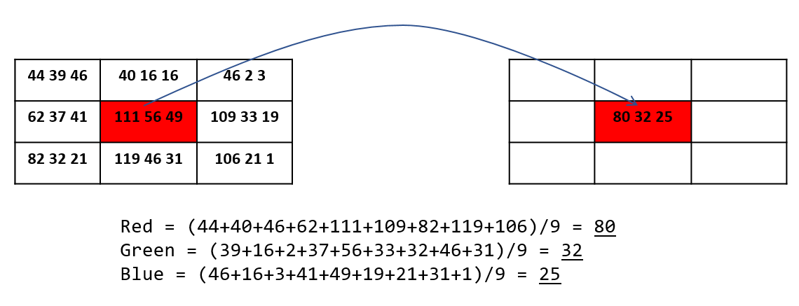
| The neighborhood of a pixel is comprised of the eight pixels that surround it. |
This is probably best handled by writing a function that takes a surface and an \((x,y)\) coordinate and returns an RGB triple that is the average color of \((x,y)\) and all of its neighbors. Using our box and arrow notation we have …
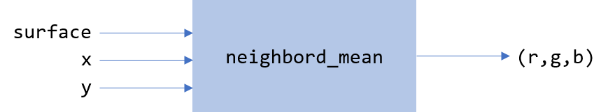
neighborhood_mean of a pixelThe function header should be …
1
2
def neighborhood_mean(surf, x, y):
pass (1)
| 1 | Recall that we use the pass statement as a placeholder for the function body. |
We could, write nine separate get_at calls to get the color of each pixel, this is a bit tedious and not very general. Notice how the nine pixels form a 3 X 3 grid. If \((x,y)\) represents the center pixel in the grid, then the row above is \(y-1\) and the row below is \(y+1\). The column to the left is \(x-1\) and the column to the right is \(x+1\). We can use our nested for-loop pattern to go through the 3 X 3 grid.
1
2
3
4
5
6
7
8
9
10
11
12
13
14
15
16
17
18
def neighborhood_mean(surf, x, y):
red_sum = 0 (1)
green_sum = 0
blue_sum = 0
for ny in range(y-1,y+2): (2)
for nx in range(x-1,x+2): (3)
(r,g,b,_) = surf.get_at((nx,ny)) (4)
red_sum += r (5)
green_sum += g
blue_sum += b
red_avg = int(round(red_sum/9)) (6)
green_avg = int(round(green_sum/9))
blue_avg = int(round(blue_sum/9))
return (red_avg, green_avg, blue_avg)
| 1 | Local variables to keep the sum of each color component. |
| 2 | For each row in the 3 X 3 grid. Why y+2 and not y+1? |
| 3 | For each column in the 3 X 3 grid. Why x+2 and not x+1? |
| 4 | Get the neighborhood pixel color components. |
| 5 | The notation var1 += var2 is shorthand for var1 = var1 + var2. So red_sum += r means red_sum = red_sum + r. |
| 6 | A color component must be an integer and averages are not integers; so round and convert to the closest integer. |
Now all that is left is to call neighborhood_mean for every pixel in the image, and write each pixel to an initially empty surface. We might best think of this as a function mean_filter that takes a surface and returns a new surface.
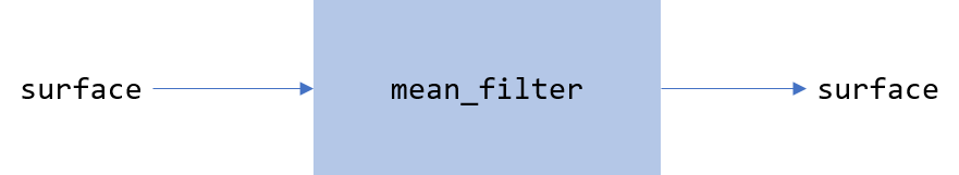
There is one issue to contend with? What do we do about the pixels along the border? For instance, the pixels along the left edge don’t have any neighbors on the left and if the neighborhood_mean functions tries to access a negative x coordinate the program will crash.
There are several ways we could handle this. We could modify neighborhood_mean to not access pixels outside of the boundary of the image, and only compute the mean of the neighbors the pixel does have. Pixels along the left edge (except the corners) would only have five neighbors. Corner pixels only have three neighbors, etc. We would have to keep a count of the number of actual neighbors because we can’t always divide by nine.
An easier way is to skip over the border pixels and skip the first and last row and column.
1
2
3
4
5
6
7
8
9
def mean_filter(orig):
surf = pygame.Surface((orig.get_width(), (1)
orig.get_height()))
for y in range(1,orig.get_height()-1): (2)
for x in range(1, orig.get_width()-1): (3)
(r,g,b) = neighborhood_mean(orig, x,y) (4)
surf.set_at((x,y), (r,g,b)) (5)
return surf (6)
| 1 | Create the new surface for the filtered image |
| 2 | Check the loop bounds. We are skipping the first and last row of pixels. Why? |
| 3 | Skipping the first column and last column of pixels. Why? |
| 4 | Call the nighborhood_mean function from above. |
| 5 | Write the new pixel to the new surface. |
| 6 | Don’t forget to return the new surface. |
Here is the original enlarged, pixelated, image.
And here is the filtered version.
The beautiful thing about writing this as a fuction is that if we wanted to filter the image twice we can just use function composition and call mean filter two or three times.
filtered_image = mean_filter(
                     mean_filter(
mean_filter(image)))Complete the main program that calls mean_filter on an image.
import pygame, util
pygame.init()

image = pygame.image.load("rainbow_toad_enlarged.png")

win = pygame.display.set_mode((image.get_width(), image.get_height()))
win.blit(image, (0,0))
pygame.display.update()

print("Click to continue")
util.wait_for_click()

surf = mean_filter(image)

win.blit(surf, (0,0))

pygame.display.update()

print("Click to continue")
util.wait_for_click()
10.6. Image file formats
Computer and software manufactures have defined various techniques for storing images in files. These techniques usually allow the image to be compressed so that it uses less storage.
We have already seen one way we can compress an image - just make it smaller. Our scale function does this. It is not a terribly great way to compress an image but lots of software does this. For example, when you take a picture with your phone and then text it to someone, the texting software will usually shrink the image to reduce data consumption on your cellular plan. This kind of compression just throws some of the pixels away, it loses information.
| With lossy compression data is either discarded or modified and cannot be reconstructed from the compressed data. |
Lossy compression is often acceptable. For example, the JPEG image format uses lossy compression (albeit in a far more sophisticated way than just leaving pixels out), and as long as the image still looks good we tend not to care. Audio file formats such as mp3 also use lossy compression.
| JPEG (Joint Photographic Experts Group [24]) uses advanced mathematics to achieve good, but lossy, compression. |
Sometimes lossy compression is not acceptable. For example, what if we wanted to compress a large word processing document. We couldn’t have the compression technique modify or throw away characters. Compression techniques that do not lose information are called non-lossy or lossless.
The Portable Network Graphics image format (PNG) uses lossless compression. The lossless compression techniques are too advanced to discuss here, but we can give an example of a simple technique. What if an image contained a sequence pixels that were all the same color. For example, a white background might have a 100 white pixels (or 300 hundred integers that were all 255). Rather than just repeat the value 255, three hundred times, we could somehow record this in the file as \(255(300)\). This lossless scheme is called run length encoding, because it encodes long runs of the same number as two integers, the number to be repeated and then number of times it needs to be repeated.
| PNG [25] One of the techniques used in PNG’s lossless compression is called Huffman Encoding, a common technique discussed in a Data Structures text. |
PNG and JPEG are probably the two most important image file formats, but there are other popular formates including GIF (Graphics Interchange Format), and BMP (Bitmap file format).
The moral of the story is that image file formats that use lossy compression (i.e., JPEG) will change the values of the colors in your file. For example, if you set a pixel to the color value (23,99,140) if might get changed when the file is saved as a JPEG to some other "nearby" value such as (24,98,141).
|
10.7. Secrets
As an exercise lets go through every pixel in the image of the red panda below, and if the red component of the pixel is odd, then color the pixel black. If it is even then color the pixel white.

https://commons.wikimedia.org/wiki/File:Panda_minore_(Ailurus_fulgens).JPG| When you right click on the image and save it, note that it is a PNG file. Make sure to save it as a PNG file. |
In previous examples we have loaded the image on a surface, processed the surface, and then blitted the image surface on the display surface. In this particular case let me suggest that we immediately blit the image to the display, and process the display surface. This will add a bit of dramatic effect.
1
2
3
4
5
6
7
8
9
10
11
12
13
14
15
16
17
18
19
20
import pygame, util, color
pygame.init()
image = pygame.image.load("red_panda.png")
win = pygame.display.set_mode((image.get_width(),
image.get_height()))
win.blit(image, (0,0)) (1)
pygame.display.update()
for y in range(win.get_height()):
for x in range(win.get_width()):
(r,g,b,_) = win.get_at((x, y))
if r % 2 == 1: (2)
win.set_at((x, y), color.black) (3)
else:
win.set_at((x, y), color.white)
pygame.display.update() (4)
pygame.time.delay(5) (5)
util.wait_for_click()
| 1 | Show the image of the red panda. |
| 2 | If the red component is odd make the pixel black, otherwise white. |
| 3 | Because we want to animate this process we are modifying the display surface and not the image surface. This required, of course, that the image was already blitted to the display. |
| 4 | Inserting the display update here will update the display after every row is modified. This is necessary for animation. What would happen if we indented this line one level to be inside the inner for-loop? |
| 5 | This delay is for dramatic effect only. |
After running this code on the image of the red panda you’ll see a secret hidden message.
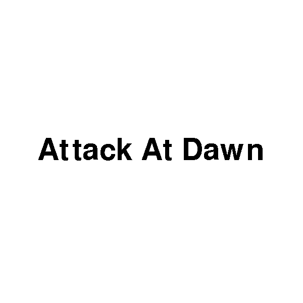
10.7.1. Hiding a message in an image
This seems a bit creepy, but notice that the message is black-and-white. From our program above we see that the message is hidden in the odd red pixels. Lets figure out how we could hide a message in an image. The first thing we need to do is "make room" for the secret message. What if we were to preprocess an image and change the red component of each pixel so that it was even. For instance, if the red component of a pixel was 201, we change it to 200. That will not have a noticeable visible effect on the image, even if we ended up changing every pixel.
Why is it important that we subtract one and not add one to make a pixel even?
The red component could be 255, adding one would make it 256, which would cause a run-time error indicating that a color value was out of range.
Write a function that takes a surface and sets all of the red pixels to even values that are at most one less than their original value.
1
2
3
4
5
6
7
def make_red_even(image):
for y in range(image.get_height()): (1)
for x in range(image.get_width()):
(r, g, b, _) = image.get_at((x, y))
if r % 2 == 1: (2)
image.set_at((x, y), (r - 1, g, b)) (3)
return image
| 1 | We should be getting comfortable with this nested for-loop pattern for accessing each pixel on a surface. |
| 2 | This checks to see if the red component is odd. |
| 3 | If it is odd, then decrease the red value by one and set it. |
Notice that make_red_even does not create a new empty surface but modifies the original surface passed in. Recall that objects passed in as a parameter (such as the surface image) are really a reference to the object. We could, if we wanted, have created a new, initially empty surface, with new RGB values, leaving the original image unmodified. When we should create a new surface object or modify an existing one is subtle, and there are no hard and fast rules. In this particular case I wanted to show that you can modify an object through its reference parameter.
Now we have an image where all of the red values are even. What if we were to create another image of exactly the same dimensions that is pure black-and-white (no intermediate gray values) that contains a secret message. There are many ways to create a black-and-white image with text in it. You can use an image editing program such as Photoshop, Gimp, or Microsoft Paint. But probably the easiest way to do it is programmatically, directly in Pygame.
The following two lines create a surface with the text Attack At Dawn rendered on it.
my_font = pygame.font.SysFont("Veranda", 48) (1)
secret = my_font.render("Attack At Dawn", False, color.black) (2)| 1 | Create a font object, with 48pt text size. If the font Veranda is not on the system Pygame will use a default font. |
| 2 | Create a surface with the text Attack At Dawn on it using the color black (the third argument). The boolean value False means do not use antialiasing to smooth the edges on the text, but we want the image to be pure black-and-white, so we don’t antialias. |
| Antialiasing uses shades of a color to smooth edges. |
You can see the difference with anti-aliasing in the image below. The text on top does not use anti-aliasing while the text on the bottom does. You notice the difference the most where the edges of the letters are either curved or at an angle.
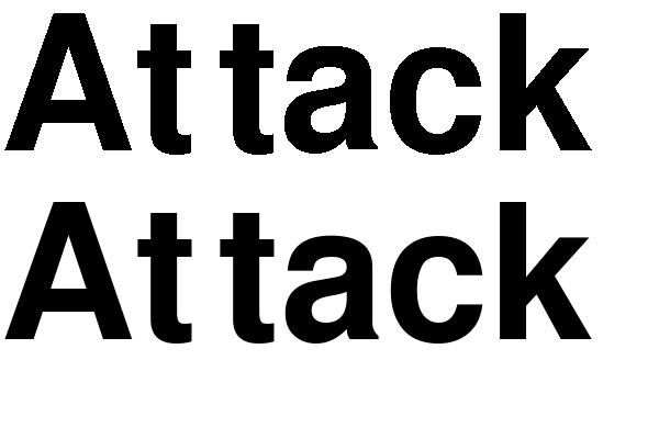
Now that we have 1) a surface with a secret message on it, and 2) an image where all of the red values are even we need to go through each pixel in the secret message, check to see if it is black, and if it is black, make a corresponding pixel in the original image odd. Assume we are putting the secret message in the upper left hand corner of the image so that coordinate \((0,0)\) in the image corresponds with coordinate \((0,0)\) in the secret message surface. We can think of this as overlaying the secret message on the window. We are making a big assumption that the message surface will fit in the image. That is, both the message width and height are less than the image width and height.
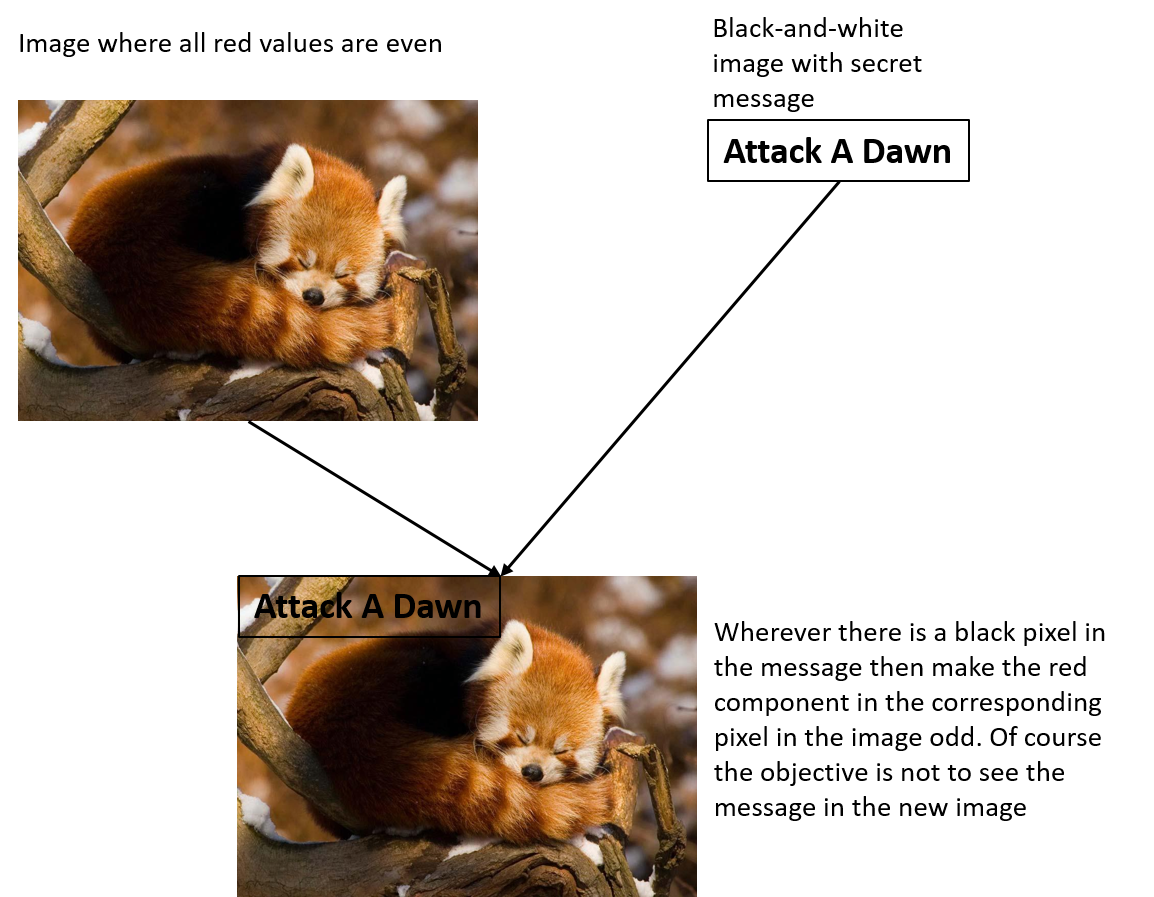
The following program hides a message in an image putting everything together.
encrypt.py 1
2
3
4
5
6
7
8
9
10
11
12
13
14
15
16
17
18
19
import pygame,util,color
pygame.init()
# Main Program
image = pygame.image.load("some_image.png") (1)
image = make_red_even(image) (2)
font = pygame.font.SysFont("Veranda", 40)
msg = font.render("Python is Awesome", False, color.black) (3)
for y in range(msg.get_height()): (4)
for x in range(msg.get_width()):
(r,g,b,_) = msg.get_at((x,y)) (5)
if (r,g,b) == color.black: (6)
(ir,ig,ib,_) = image.get_at((x,y)) (7)
image.set_at((x,y), (ir+1,ig,ib)) (8)
pygame.image.save(image, "new_image.png") (9)
| 1 | Make sure the image is a PNG. Why? Because of lossless compression. |
| 2 | Call the make_red_even function. |
| 3 | Create a secret message Python is Awesome |
| 4 | Go through each pixel in the secret message. |
| 5 | Get the message pixel and … |
| 6 | Check if it is black. |
| 7 | If it is black then we need to get the corresponding pixel in the image and … |
| 8 | make the red component f the image pixel odd. Hence the ir+1. |
| 9 | pygame.image.save is a new Pygame function that saves a surface in a new file in the image format specified by the file suffix. In this case it saves the surface image in the file named new_image.png as a PNG file because the file name ends with .png. |
| The above program can crash if the image containing the message is larger than the image that is hiding the message. |
Look at how we check if a color is black on line 15.
if (r,g,b) == color.black:
...This is checking using tuple equality by comparing each value in the (r,g,b) tuple against the tuple specified in color.black which is (0,0,0).
Comparing tuples like this is handy, but if you didn’t know about tuple equality you could do this another way using logical and.
if r == 0 and g == 0 and b == 0:
...Finally, since we are certain that the message contains only black (0,0,0) or white (255,255,255) pixels, we could get away with just comparing one of the components, instead of
all three.
10.8. Case Study: Schelling’s Segregation Model
In 1969 and 1971 the economist Thomas Schelling published two now famous papers, Models of Segregation.[26] and Dynamic Models of Segregation.[27]. One of the phenomena that Schelling was trying to study was why people segregated based on race. Why people segregate by race may seem obvious; racial segregation and racism have a long, violent, and sorrowful history in America. What Schelling was trying to understand though is what might happen if we started with some sense of racial balance. Would societies continue to segregate? Schelling wasn’t just interested in race, but cited examples of all kinds of segregation such as income, sex, and educational background.
Consider the following map of New York City.

In this map each red dot represents a Caucasian household, blue represents a black household, yellow a Latino household, and green an Asian household. The segregation is obvious.
Reasons for segregation are varied and complex. Schelling tried to abstract away (that’s what a model does) details and propose something much more simple. People are agents living on a grid and follow some simple rules. People generally have choices of where they might live; if they don’t like where they are currently living they can move.
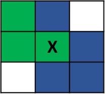
In this grid we have green agents and blue agents. White represents empty locations on the grid where agents can move. Schelling suggested that there is a threshold of the number of unlike neighbors an agent might tolerate before they decide to move. In this case we have a green agent marked with an X who is deciding if they should move. There are two empty cells, so X has six neighbors, two of which are like them, or \(2/6 = 1/3 = \overline{.33}\). If the threshold were if less than \(1/3\) of my neighbors are like me then I’ll move. In this case X would stay put. On the other hand if the threshold were \(1/2\) then X would move.
How should we pick a place to move? In this case there are two choices, the lower left cell or upper right cell. We could be smart about it and search for an empty cell that meets the threshold, in which case the lower left cell would be the place.
If X moves to the lower left we have
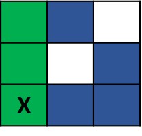
In this case X now has \(1/2\) half its neighbors like them. But what if they moved to the upper right?
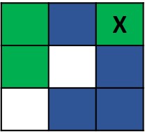
Here X now has 0 neighbors like them, and they will most likely move again in the next round.
Keeping in mind that empty cells could be far away on a large grid and not necessarily a neighboring cell, we might try for something simpler and search for an empty cell at random. It turns out either method will work. But from what Python we know now, choosing a cell at random is the easier solution.
The scenario just discussed for X is just one cell. We need to repeat this process for every cell in the grid. But when should we stop the process? When all agents are "happy" and we have no more agents moving. The question is what do we think will happen in the long run? Even with a relatively low threshold such as \(1/3\)?
In pseudocode here is the process we outlined:
-
Randomly populate a grid with roughly equal numbers of green and blue agents and empty cells.
-
Repeat until no more cells move
-
For each cell \((x,y)\) in the grid
-
if \((x,y)\) is an empty cell then continue on to the next cell
-
Otherwise count the like neighbors of cell \((x,y)\)
-
if the threshold is not met then search for an empty cell and move there
-
-
To tackle the complexity of writing this program lets try and break this down into some functions. For step 1 lets write a function randomly_populate that takes a surface and randomly assigns each cell to be one of green, blue, or empty (white) with equal probability. (We could also modify this so that one color is less populated than another).
For step 2.a.ii we can write a function like_neighbors that, given an agent’s coordinate, counts the number of neighbors that are like that agent. This should feel familiar; reminiscent of the neighborhood_mean function where we looked at the neighbors of a pixel.
For step 2.a.iii lets write a function find_empty that finds an empty cell.
10.8.1. Step 1: Randomly populate
The function randomly_populate fills the grid with blue, green, or empty (white) agents (pixels).
1
2
3
4
5
6
7
8
9
10
def randomly_populate(grid): (1)
for y in range(grid.get_height()):
for x in range(grid.get_width()):
r = random.random() (2)
if r < 1/3: (3)
grid.set_at((x, y), color.blue)
elif r < 2/3: (4)
grid.set_at((x, y), color.green)
else: (5)
grid.set_at((x, y), color.white)
| 1 | Modify grid through its reference rather than create a new empty surface. |
| 2 | A random float between 0 and 1. There is a reason we are using random() here
and not randrange(). Later on it will be easier to make the populations of agents different, for example 25% green and 50% blue. |
| 3 | Cell is a blue agent with 1/3 probability \((0 < r < 1/3)\). |
| 4 | Cell is a green agent with 1/3 probability \((1/3 < r < 2/3)\). |
| 5 | The remaining \(1/3\) are empty cells. |
If we were to run randomly_populate we will end up with a starting grid that might look something like the following, equal parts green, blue, and white.
10.8.2. Step 2: Count like neighbors
In the Schelling model we need to count the number of neighbors of an agent that are like (the same color as) that agent. For a given agent at coordinate \((x,y)\) we will have count_like_neighbors return the proportion of the eight neighboring agents that are like agent at coordinate \((x,y)\). What should we do about empty cells? Presumably an agent neither likes nor objects to being adjacent to an empty cell, so we will not count them as a neighbor. Consequently, if there is one empty neighbor, and there are two like neighbors our function should return return \(2/7\).
1
2
3
4
5
6
7
8
9
10
11
12
13
14
15
16
17
18
def count_like_neighbors(x,y,c,grid): (1)
like = 0 (2)
nc = 0 (3)
size = grid.get_width() (4)
for row in range(y-1, y+2): (5)
for col in range(x-1, x+2): (6)
(r,g,b,_) = grid.get_at((row % size, col % size)) (7)
if (r,g,b) != color.white: (8)
nc = nc + 1
if (r,g,b) == c: (9)
like = like + 1
if nc == 0: (10)
return 0
else:
return (like-1)/nc (11)
| 1 | (x,y) is the coordinate of the current agent. Presumably c is blue or green because we should not be counting the neighbors of an empty cell. |
| 2 | Local variable like will be the count of the number of like neighbors. |
| 3 | Local variable nc, or neighbor count, will be the count the number of non-empty neighbors. |
| 4 | Local variable size is the width and height of grid. |
| 5 | This loop pattern we have seen before for looking at the neighbordhood of a cell. row ranges from the row above the agent to the row below. |
| 6 | col ranges from the column to the left of the agent to the column to the right. |
| 7 | We are calculating the coordinate mod size which means we are wrapping around the edges. This is just an easy way to avoid checking for out of bounds conditions. |
| 8 | If the neighbor is not empty then increment the neighbor count. |
| 9 | If the neighbor color is the same as the agent then increment the like count. |
| 10 | If there are no neighbors then return zero, otherwise we run the risk of dividing by zero. |
| 11 | We are subtracting one from like because the agent at (x,y) counted itself. |
| We always need to watch out for dividing by zero. |
Function count_like_neighbors is a little subtle. We had to be careful about dividing by zero and and an agent not counting itself as a like neighbor.
10.8.3. Step 3: Finding an empty cell
When an agent moves it needs to find an empty cell to move to. We could search for an empty cell in one of several ways, we could just start looking for an empty cell in the grid starting at the top and working our way down using our nested for-loop pattern. This would give preference to empty cells towards the top and slowly fill in the grid entirely from the top.
Alternatively, we could randomly search for an empty cell. If, for example, one third of the cells are empty then it would take, on average, three random searches to find an empty cell.
Function find_empty randomly searches for an empty cell in the grid returning its coordinate when it has found one.
1
2
3
4
5
6
7
def find_empty():
while True: (1)
x = random.randrange(grid.get_width()) (2)
y = random.randrange(grid.get_height())
(r,g,b,_) = grid.get_at((x,y))
if (r,g,b) == color.white: (3)
return (x,y)
| 1 | It looks like this loop will run forever, but the function actually returns, breaking out of the loop when an empty cell is found. |
| 2 | Generate a random coordinate. |
| 3 | White means empty, so return the coordinate. |
10.8.4. Putting it all together
With function randomly_populate, count_like_neighbors, and find_empty we can put together the main program for the Schelling Segregation model. If we make the grid too large then the simulation can take a long time to run, so we will keep it as a square grid 400 on a side.
1
2
3
4
5
6
7
8
9
10
11
12
13
14
15
16
17
18
19
20
21
22
23
24
25
26
27
28
pygame.init()
n = 400
grid = pygame.display.set_mode((n,n))
randomly_populate()
threshhold = 1/3
done = False
while not done:
moved = 0 (1)
for y in range(grid.get_height()): (2)
for x in range(grid.get_width()):
(r,g,b,_) = grid.get_at((x,y)) (3)
if (r,g,b) != color.white:
like = count_like_neighbors(x,y,(r,g,b)) (4)
if like < threshold: (5)
(ex,ey) = find_empty() (6)
grid.set_at((ex,ey), (r,g,b)) (7)
grid.set_at((x,y), color.white) (8)
moved = moved + 1 (9)
pygame.display.update() (10)
print(moved) (11)
done = (moved == 0) (12)
util.wait_for_click()
| 1 | Keep processing the grid until there are no more moves (every agent is happy) |
| 2 | Go through the entire grid using our normal nested for-loop pattern. |
| 3 | Get the agent at the cell, which could be no agent (empty cell). |
| 4 | If the cell is not empty then we have an agent and get the proportion of their like neighbors. |
| 5 | If the proportion is less than the threshold then the agent needs to move. |
| 6 | Find an empty cell for the agent to move to. |
| 7 | Put the current agent at the empty location. |
| 8 | Make the agent’s old coordinate empty. |
| 9 | Increment the moved count |
| 10 | Update the display to animate the progress of the model |
| 11 | print the number of agents that moved. This should be decreasing. |
| 12 | A little trick, but this sets done to True if moved is 0. Could have used an if-statement. |
When we run the Schelling model with equal proportions of agents and a threshold of \(1/3\) we notice that there is segregation.
If we make one of the agents a minority the results are even more pronounced. Below we have 25% of the agents are blue, 50% are green, and 25% empty cells.
These results were pretty surprising. If fewer than 33% of an agent’s neighbors are like them then the agent moves with the end result being a fair amount of segregation. That is, with fairly tolerant agents, we see segregation.
One thing to check with any model is to see if it matches our intuition. If we lower the threshold, that is we make the agents even more tolerant, then we should see less segregation. This is indeed the case.
If we increased the threshold to say 50% and also introduce a minority agent population we should see even more dramatic segregation. And we do.
If, however, we make agents very intolerant by having, say a 70% threshold, and we have enough diversity in the population it can be very hard to please an agent and the simulation doesn’t every really settle down.
10.8.5. Schelling Summary
The Schelling Model was one of the early models in an area called Agent Based Modeling.[29] In Agent Based Models, agents live on a grid and are endowed with a set of rules or behaviors that dictate how agents interact with neighboring agents. There are many applications of agent based modeling across the social and natural sciences including epidemiological models of the spread of disease, predator-prey population models, and animal flocking. Later on we will see an agent based model for simulating a forest fire. While using Python and Pygame for agent based modeling is pretty effective there are special purpose programming languages designed specifically for building agent based models, NetLogo being the most prominent.[30].
11. String and File Processing
Lots of software processes text. We use word processors to edit text and write documents, web browsers to read and process text entered in web forms, e-mail clients to read and write emails. Web search engines such as Google, store and search massive amounts of text from every publicly accessible web site in the world. It is estimated that Google has exabytes of data. Biologists use tools such as BLAST to process DNA sequences that are represented as text. The IDE we use to write our Python programs and spell checkers process text. One of the most important applications of text processing is cryptography.
We have already used text in our programs; strings are text. We hardcode text into our programs using string constants …
s = 'antidisestablishmentarianism'and use them in prompts or enter them from the keyboard.
s = input("Enter a string: ")For the following discussion lets assume that s is the string 'antidisestablishmentarianism'
We can get the length of a string using the function len. The statement
print(len(s))would print 28 on the console.
We can also access individual characters in a string. The characters in a string are numbered starting with 0. We use a bracket notation for accessing individual characters. s[0] is the first character or 'a' and s[27] is the last character, or 'm'.
1
2
3
# What would get printed?
s = 'antidisestablishmentarianism'
print(s[0], s[11], s[len(s)-1])
a b mYou need to be careful about off-by-one errors.
1
print(s[len(s)])
would create an index out of range error, because it is trying to print character s[28] but that character does not exist. Oddly enough you can index from that end of the string. s[-1] is the last character, s[-2] is the second to last character, etc.
11.1. String operations
There are typically two ways we will loop through and examine each character in a string.
Assume that the variable s contains a string value. Back when we introduced the for-loop we noted that strings were a sequence type and that we can use a sequence type in a for loop.
for ch in s:
# loop bodyThe variable ch (for character) will take on each character in the string s. Lets say we wanted to count the number of times the character 'a' appeared in a string.
1
2
3
4
5
a_count = 0
for ch in s: (1)
if ch == 'a':
a_count += 1
| 1 | ch will take on each character in the string s. |
This way of looping through a string works great if you only need to look at each character independent of all the other characters.
The second way to loop through a string is to remember that each character in a string has an integer index. So another way to count the number of times the character a occurs is:
1
2
3
4
a_count = 0
for i in range(len(s)): (1)
if s[i] == 'a': (2)
a_count = a_count + 1
| 1 | i will take on the integer values 0 up to but not including 28. |
| 2 | s is a string, i is an integer, so s[i] is the character at index i. |
For example, lets say we wanted to count the number of double characters in a string. For example Mississippi has three sets of double characters; the first ss, the second ss, and the pp.
11.1.1. Strings are immutable
Once a variable has been assigned a string value, that string cannot be modified. For example, if s is a string we can’t change the value of s[0].
s[0] = 'Z'This causes an error 'str' object does not support item assignment.
| In Python strings are immutable. This means that the components of the string cannot be changed. |
The way to modify a string is to build a new one. If s1 and s2 are two strings then you can concatenate the two strings with +.
s1 = "hello"
s2 = "world"
s3 = s1 + s2
print(s3) (1)| 1 | Will print helloworld |
| To concatenate strings means to join two or more strings into one. |
11.1.2. Reversing a string
To illustrate building a string lets write a function that takes a string as an argument and returns the reverse of the string; reverse('python') is 'nohtyp'.
1
2
3
4
5
6
def reverse(s):
tmp = "" (1)
for ch in s: (2)
tmp = ch + tmp (3)
return tmp (4)
| 1 | An initially empty string that we will use to build up the reversed string (there is no space between the double quotes). |
| 2 | For each character ch in the string s. |
| 3 | This is a little tricky. We will discuss below. |
| 4 | Return the reversed string. |
Why does this work? Take the example of the string 'abcd' and follow the values of ch and tmp after each loop iteration.
ch tmp
-- ---
a a (1)
b ba (2)
c cba (3)
d dcba (4)| 1 | tmp is initially empty so the new value of tmp is ch + tmp or 'a' |
| 2 | ch is 'b' and tmp is 'a' so the new value of tmp is ch + tmp or 'ba' |
| 3 | ch is 'c' and tmp is 'ba' so the new value of tmp is ch + tmp or 'cba' |
| 4 | finally ch is 'd' and tmp is 'cba' so the new value of tmp is ch + tmp or 'dcba' |
What would happen if the loop body in the function reverse were tmp = tmp + ch instead of tmp = ch + tmp.
It just rebuilds the original string and does not build the reverse.
A palindrome is a word that reads backwards and forwards such as racecar, kayak, and madam. Write a function palindrome that takes a string as an argument and returns true if the argument is a palindrome, false otherwise. Hint: use the reverse function.
This is kind of easy if we can use the reverse function.
def palindrome(s):
if s == reverse(s):
return True
else:
return FalseThere is an even more concise way to write the palindrome function.
def palindrome(s):
return s == reverse(s)The way to think about this is that if is s is equal to reverse(s) then that is the value True, which is then returned. If they are not equal then it evaluates to False which is then returned. This is the same exact behavior as the first version of palindrome.
11.1.3. Searching a String
Often we will want to search a string for a substring. For example, does the string 'establish' appear somewhere in the string s. The string function s1.find(s2) returns the starting location of the first occurrence of the string s2 in s1. It returns -1 if it is not there.
s1 = 'antidisestablishmentarianism'
s2 = 'hippopotomonstrosesquipedaliophobia'
print(s1.find('establish')) (1)
print(s1.find('hippo')) (2)
print(s2.find('po')) (3)| 1 | prints 7 |
| 2 | prints -1 |
| 3 | prints 3, the first occurrence of 'po' |
A second version of the find function takes a starting location for the search; s1.find(s2,start) will return the location of s2 in s1 starting at index start.
print(s2.find('po', 4)) (1)| 1 | prints 5 |
If we didn’t know to start the search at 4 and we wanted to find the second location of po we can search for the first occurrence and use that as a starting point for a search for the second occurrence.
start = s2.find('po') (1)
print(s2.find('po', start+1)) (2)| 1 | index of first occurrence of po |
| 2 | start searching for the second occurrence at start+1 and not start, otherwise we would just find the first occurrence all over again. |
Write a program that reads a string from the user and counts the number of times the substring 'is' appears. Print a user friendly answer. Use the find function but do not use the built-in string function count.
1
2
3
4
5
6
7
8
9
s = input("Enter a string: ")
count = 0
loc = s.find('is') (1)
while loc != -1: (2)
count += 1
loc = s.find('is',loc+1) (3)
print('"is" appears', count, "times in",s)
| 1 | Find the first occurrence |
Here is an example execution.
Enter a string: antidisestablishmentarianism
"is" appears 3 times in antidisestablishmentarianismOkay, so we could have used the built-in string function count to do this.
print(s.count('is'))As is often the case, Python’s built-in set of functions and libraries will often have what you are looking for.
11.1.4. String Slices
The bracket notation picks out individual characters in a string;
s[i] is the character at index i. The bracket notation is also used to pick out consecutive portions of a string, a substring, using what Python calls a slice operation. The notation s[x:y] extracts the portion of the string starting at index x and up to but not including the character at index y.
s = 'antidisestablishmentarianism'The slice s[0:4] is the string 'anti'. The slice s[7:16] is the string 'establish'.
Leaving off the ending index then the slice is to the end of the string.
print(s[7:])will print establishmentarianism.
Leaving off the starting index then the slice starts at index 0.
print(s[:4])will print anti.
A common use for combining find and a string slice is when we are trying to parse data. For example, lets say we asked the user to enter two numbers separated by a comma. We will then compute the average of those two numbers. The user will enter something like '39,88'. But this will be a string, so we need to bust apart the two numbers. We can do this by finding the comma, and taking the slice before the comma, and the slice after the comma. We also have to be careful to convert the slices from strings to integers
print("Enter two numbers separated by a comma.") (1)
s = input("> ") (2)
comma = s.find(',') (3)
num1 = int(s[:comma]) (4)
num2 = int(s[comma+1:]) (5)
avg = (num1 + num2) / 2
print("Average:", round(avg,2))| 1 | Prompt on a separate line because it is a little long. |
| 2 | Prompt is short and sweet, just ">". |
| 3 | Find the position of the comma. |
| 4 | The first number is before the comma. |
| 5 | The second number is after the comma. |
Ask the user to enter three numbers separated by a comma. Print their average.
There are lots of ways to tackle this. Here is one.
print("Enter three numbers separated by a comma")
s = input("> ")
comma1 = s.find(',') (1)
comma2 = s.find(',', comma1+1) (2)
num1 = int(s[:comma1]) (3)
num2 = int(s[comma1+1:comma2]) (4)
num3 = int(s[comma2+1:]) (5)
avg = (num1 + num2 + num3) / 3
print("Average:", round(avg,2))| 1 | Index of first comma. |
| 2 | Index of the second comma. |
| 3 | First number is before first comma. |
| 4 | Second number is between the first and second comma. |
| 5 | Third number is after the second comma. |
Finally, lets take this one step further and handle an arbitrary number of integers each separated by a comma. We will need to loop through the numbers some how.
Enter numbers separated by a comma
> 2,9,12,-33,15,7,99
Average: 15.86Similar to the way we counted the number of times we search for a substring in a string.
A list of numbers separated by commas are called comma separated values. Files that contain comma separated values are often use a .csv file suffix.
|
Like always, there are lots of different ways we could write this, but one way to think about this is to repeatedly get the first number in the list and then remove the first number in the list, thereby making the second number the new first number. Lets say the user entered 23,19,46,57 into the string s. We also need to keep a running total of the numbers and the count of the number of integers. We will use total and count for that.
s total count
----------- --- -----
23,19,46,57 0 0 (1)
19,46,57 23 1 (2)
46,57 42 2 (3)
57 88 3 (4)
145 4 (5)| 1 | s is the original input CSV list. |
| 2 | Extract the first number 23, add it to total, increment count, and delete 23. |
| 3 | Extract the first number 19, add it to total, increment count, and delete 19 |
| 4 | Extract the first number 46, add it to total, increment count, and delete 46. |
| 5 | We should be seeing a pattern here. Extract the first number 57, add it to total, increment count, and delete `57. Compute a final average of \(145/4 = 36.25\) |
1
2
3
4
5
6
7
8
9
10
11
12
13
14
15
16
print("Enter a comma separated list of numbers")
s = input("> ")
comma = s.find(',')
total = 0 (1)
count = 0 (2)
while comma != -1: (3)
num = int(s[:comma]) (4)
total += num
count += 1
s = s[comma+1:] (5)
comma = s.find(',') (6)
avg = total/count
print("Average: ", round(avg, 2))
| 1 | To hold the running total of the numbers. |
| 2 | Keep a count of the integers entered. |
| 3 | Keep processing the list of numbers until there are no more commas. |
| 4 | Extract the leading number in the list, add it to total, and increment count. |
| 5 | Delete the leading number in the list. |
| 6 | Get the location of the next comma. |
There is actually a subtle bug in the code above; a classic off-by-one error. There are no syntax errors and the code doesn’t necessarily crash (more on that later) but it does produce an incorrect result. For example, if we enter 23,19,46,57 we get an average of 29.33. Recall the answer should be 36.25.
Find and fix the bug in the above code.
The problem is that we skip the last number. For example, if we have the original list
23,19,46,57 eventually the list becomes 57 after line 12. There are no more commas in the list
so on line 13 comma becomes -1 and when we go back to check the loop condition the loop will quit having not processed the 57. An easy fix is to realize that after the loop terminates s now contains the final number in the list. Add it to total, and don’t forget to increment count. The code after the loop becomes:
total = total + int(s) (1)
count += 1 (2)
avg = total/count
print("Average: ", round(avg, 2))| 1 | Add the final number to total. COuld we have used num here and not s? No. Why? |
| 2 | And increment count. |
One more thing to check is to make sure the code works if we only have a single number to start with. This was also a problem before we fixed the bug, but now works.
11.1.5. Error Checking
The term hacker used to be a badge of honor. It just meant you were a sharp programmer. The term now has a negative connotation and usually refers to someone using there technical skills unethically and possibly illegally. Hackers either break into systems to steal information, plant virus' or cause an organization’s software systems to crash.
We will talk a little bit about breaking in to systems when we discuss cryptography so lets talk about possibly causing software to crash. One way to try and cause a software system to crash is to enter bogus data in the input. We have all seen this before when we enter data into a web form. If we forget to enter a zip code in our address then the system will generally not let us proceed. Up until we know we haven’t talked about checking the input data for errors, or error checking, but it is worth a cursory discussion.
Lets look at our above example of computing the average of a list of numbers. What if instead of a list of numbers we entered an ill-formed line such as rumpelstiltskin, or 23,16,fred,11. We get a run-time error (what I have also been calling a crash).
ValueError: invalid literal for int() with base 10: 'rumpelstiltskin'
This makes sense, Python does not know how to convert rumpelstiltskin to an integer. I’d be worried if it did. Error checking is a little too advanced for us to cover now, but real software systems have to always check inputs for erroneous data to keep a system from crashing. In this case it would entail adding code to check and make sure that the user really entered a well formed list of integers separated by commas. If there was a problem the program could exit gracefully or the program could keep asking until the user entered something valid.
11.1.6. Example: Word scramble
Lets say we were implementing a word scramble game where we present the user with an anagram and ask them to to try and guess the word. For now we will hard code the word they are trying to guess in the game.
| An anagram is a rearrangement of the characters in a word. |
Like always, lets break this up in to subproblems. Lets write a function scramble that takes a string and returns a random anagram of that string. For example scramble('python') might return 'hotpyn' or toyhpn.
What are the chances that scramble will return the original word? Well for python there
are six distinct characters and the first character in the scrambled word could be any of the 6. The second character could be any of the remaining 5. The third character any of the remaining 4, etc. This gives us \(6\cdot5\cdot4\cdot3\cdot2\cdot1 = 720\) different possibilities for the word python. In general if a word has \(n\) distinct characters then there are at least \(n\) factorial (denoted as \(n!\)) permutations of the characters in the word. So the probability is \(1/n!\).
|
We repeatedly pick a random character from the word, and append the character to our scrambled word. We also need to be careful that we delete the chosen character from the word so we don’t choose it again. So something like, the following process. Assume our word is in a string word and our new scrambled word is being constructed in a variable tmp. Lets also assume the a variable i contains a random index into word.
word i tmp
----- - ---
python 5 n (1)
pytho 3 nh
pyto 0 nhp
yto 1 nhpt
yo 1 nhpto
y 0 nhptoy
(2)| 1 | tmp initially starts out as the empty string. |
| 2 | At this point the len(word) is 0 so the loop terminates. |
Here is the function scramble.
1
2
3
4
5
6
7
8
9
def scramble(word):
tmp = ''
while len(word) > 0:
i = random.randrange(len(word)) (1)
tmp += word[i] (2)
word = word[:i] + word[i+1:] (3)
return tmp
| 1 | Choose a random index into the word. |
| 2 | Concatenate the character at that index into our temporary string tmp. |
| 3 | Deletes the character at index i by rebuilding the word with all of the characters before index i (word[:i]) concatenated with all of the characters after index i (word[i+1:]). |
Putting it all together we have:
1
2
3
4
5
6
7
8
9
word = 'python' (1)
anagram = scramble(word)
print(anagram)
guess = input('Enter word: ')
if guess == word:
print("Correct")
else:
print("Incorrect. The word is", '"' + word + '"')
| 1 | Okay, it is a little silly to have a word scramble game with one word. We will fix that next. |
11.2. Files
Up until now all of the input to our programs has come from the command line. It is common though that data come from a separate text file. Revisiting our word scramble game, lets assume we have a text file of words, one word per line, and the file is named words.txt. We will keep it relatively short for now, but files can be enormous and could have hundreds of thousands of lines it.
apple
banana
interpreter
racoon
zombie
example
incorrectThe first thing to know is that every line ends with a special character that you cannot see called the end-of-line character a.k.a. newline character. We often call spaces, tabs, and newline characters whitespace characters. In most programming languages the newline character is written \n.
f = open('words.txt') (1)
# process the file
f.close() (2)| 1 | If words.txt doesn’t exist then you will get an error indicating that the file was not found. |
| 2 | After we are done with the file it is a good practice to close the file by calling the function close on the file object returned from open. |
Function open takes a string as an argument that is the filename to be opened and it returns a reference to a file object. In this case being assigned to the variable f (like always we could have used any variable name here).
There are various ways we can read the data in a file, probably the most straightforward is to read it line-by-line using a for-loop. Recall that in a for-loop we need a variable that represents a sequence type, and it turns out a file object is such a type. For instance,
1
2
for line in f: (1)
print(line)
| 1 | f should be the variable from the call to open. |
This will read and print each line in the file to console. But the output is not what you might expect for words.txt.
apple
banana
interpreter
raccoon
zombie
example
incorrectWhy is there a blank line between each word?
Recall that every time print is called the last character printed is a newline character \n. But also recall that there is a newline character after every word in the file. So we end up printing two newline characters.
We can fix this in two ways. The first way is to slice off the last character in the line (the newline character) before we print it.
for line in f:
print(line[:len(line)-1]) (1)| 1 | Why len(line)-1 instead of len(line)? |
Or we can tell the print function to suppress printing a newline character using a named parameter.
for line in f:
print(line, end='') (1)11.2.1. Counting the lines in a file
How can we count the lines in a file?
1
2
3
4
5
6
7
8
f = open('words.txt')
count = 0
for line in f: (1)
count += 1
f.close() (2)
print("words.txt has", count, "lines")
| 1 | Notice that we are not even using the variable line in the code. |
| 2 | Recall that it is a good practice to close the file when we are done. |
Once again, this is probably better provided as a reusable function.
1
2
3
4
5
6
7
8
9
10
11
def linecount(fname):
f = open(fname)
count = 0
for line in f:
count += 1
f.close()
return count
# Main program
name = 'words.txt'
print('File', name, 'has', linecount(name), 'lines')
Function linecount takes the name of a file as a parameter and returns the number of lines in that file.
11.2.2. Word Scramble using a file
Our previous version of word scamble used a single hard coded word that the user had to guess. Not very interesting. We can now go through the file of words and let the user play multiple times.
1
2
3
4
5
6
7
8
9
10
11
12
13
14
words = open('words.txt') (1)
for word in words: (2)
if word[len(word)-1] == '\n': (3)
word = word[:len(word)-1]
anagram = scramble(word)
print("What word is this an anagram of?", anagram)
guess = input('Enter word: ')
if guess == word:
print("Correct")
else:
print("Incorrect. The word is", '"' + word + '"')
break (4)
| 1 | The variable that refers to the file object does not have to be named f, in this case we are calling it words. |
| 2 | And the for-loop variable does not have to be named line, in this case word makes sense. |
| 3 | This is a little tricky. We need to remove the end of line character '\n', but the last line in the file doesn’t have an end-of-line character but an end of file character. |
| 4 | The break statement causes the for-loop to terminate. More specifically it breaks out of the innermost enclosing for or while loop. |
11.3. Example: Bioinformatics
DNA, Deoxyribonucleic Acid, is a molecule that caries the genetic information of all living organisms. DNA has a helical structure famously described by Watson and Crick.[33]
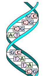
DNA in one respect can be consider a digital code because a DNA strand can be abstractly represented as a string of characters a, c, g, and t. These stand for the nucleotides (sometimes called base pairs) adenine, cytosine, guanine, and thymine respectively. For example the start of the DNA sequence for the Escherichia coli (abbreviated E. coli) bacteria is
agcttttcattctgactgcaacgggcaatatgtctctgtgtggattaaaaaaagagtg ...
It doesn’t look like this means much but this sequence of nucleotides means something to a molecular biologist and can be analyzed using a computer. Not surprisingly programs on strings play an important part of this analysis.
| Bioinformatics is the computational branch of molucular biology. |
We can start with a simple example. One quick question we could answer are some basic statistics about the sequence. How many occurrences of each nucleotide are there? What are the relative frequencies of the nucleotides in E. coli as a percentage?
1
2
3
4
5
6
7
8
9
10
11
12
13
14
15
16
17
18
19
20
21
22
23
24
ecoli = open("ecoli.txt") (1)
a_count = 0
c_count = 0
g_count = 0
t_count = 0
for line in ecoli: (2)
for bp in line:
if bp == 'a': (3)
a_count += 1
elif bp == 'c':
c_count += 1
elif bp == 'g':
g_count += 1
elif bp == 't':
t_count += 1
total = a_count + c_count + g_count + t_count
print('length:', total)
print('a: ', a_count, ', ', round(a_count/total * 100, 1), '%', sep='') (4)
print('c: ', c_count, ', ', round(c_count/total * 100, 1), '%', sep='')
print('g: ', g_count, ', ', round(g_count/total * 100, 1), '%', sep='')
print('t: ', t_count, ', ', round(t_count/total * 100, 1), '%', sep='')
| 1 | Download this file by clicking on the link above in the sequence. |
| 2 | For each line in the file. (It turns out there is only one in this example.) |
| 3 | Count the base pairs in the current line. |
| 4 | We are controlling the spaces in the line manually by indicating that the separator should be the empty string. That is don’t print a space after the comma separated items in the print statement. |
After we execute the program we get the following results.
length: 4638690
a: 1142069, 24.6%
c: 1179222, 25.4%
g: 1176575, 25.4%
t: 1140824, 24.6%A few points. The number of base pairs in the sequence is approximately 4.6 million \(4.6 \times 10^6\). The computer was able to process a huge string quickly, in under a second. The second thing to notice is that it looks like there is a relationship in the relative frequencies of base pairs. For E. coli if we round these values then each base pair is about 25% of the total. Notice that c and g are both 25.4% and a and t are the same at 24.6%. This might indicate that there is some special relationship between a/t and c/g. Indeed there is. If we had this sequence but we did not know that it came from E. coli we could use GC Content to help narrow down the organism a DNA sequence comes from. For example it is known that the GC Content of E. Coli is 50.7% and that of humans is 41%.
GC Content is the ratio of the number g and c base pairs to the total number of pase pairs. GC Content is \((g + c)/(a + c + g + t)\)
|
GC Content is a simple example of how strings are used to analyze DNA. Many of the algorithms used in bioinformatics are too advanced to describe in an introductory course.
| Genomics is the branch of bioinformatics that uses string algorithms to study DNA (and RNA) sequences. |
11.3.1. Searching a DNA Sequence
The central dogma describes how DNA is converted to RNA to make proteins. A gene is a special region (or substring) of a DNA sequence that forms a basic unit of heredity. DNA sequences contain genes and are sometimes referred to a protein-coding genes. A codon is three consective base-pairs such as GCA or AAT. Protein coding genes obey the following constraints.
-
Start with the codon
ATG, (sometimes called a start codon). -
End with one of the stop codons
TAA,TAG, orTGA. -
The number of base-pairs (nucleotides) between the start and stop codons must be a multiple of three.
-
None of the intervening codons is one of the stop codons.
For example the sequence acatgcattggagctgaacca contains a potential gene (highlighted) while the sequence acatagttggagctgaacca is not. The reason is that starting at index three we have ata and not atg.
Verify that the first highlighted region above matches the criteria for a potential gene.
The highlighted region starts with the codon atg, the start codon. It ends with one of the stop codons tga. The region between the start and stop codons is cattggagc, which has nine base-pairs, a multiple of three. Since the gene must also start with a atg and end with a stop-codon that has three base-pairs, the length of the entire sequence must also be a multiple of three.
Lets write a program to find all of the potential genes in the E.coli bacteria. The program should print the starting location and the ending location of each potential gene location. For example the digram below shows that the first possible gene location starts at location 29 and ends at location 95.
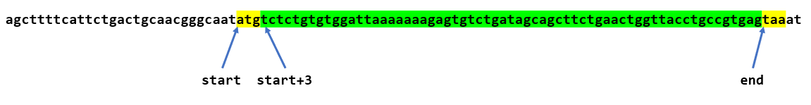
The yellow highlights are the start and stop codons. To get the started we can find the location of the first occurrence of the start codon atg and then keep looking for one of the stop codons every three base-pairs after the start codon, stopping as soon as we find one.
1
2
3
4
5
6
7
8
9
10
f = open('ecoli.txt')
dna = f.readline()
start = dna.find('atg') (1)
if start > -1: (2)
for i in range(start+3, len(dna)-3, 3): (3)
if dna[i:i+3] in ['taa', 'tag', 'tga'] and \ (4)
(i - start) % 3 == 0: (5)
print(start, i)
break (6)
| 1 | Find the location of the start codon. |
| 2 | Only look for a stop codon if we found a start codon. |
| 3 | Look for a stop codon starting from start+3 being careful not to go off of the end of the DNA string and a potential index out of bounds error. |
| 4 | This is a nice way to check for the stop codon instead of a complicated logical expression sch as dna[i:i+3] == 'taa' or dna[i:i+3] == 'tag' etc. |
| 5 | Make sure the length of the region is divisible by three. |
| 6 | As soon as we find a possible gene location stop looking because the rule is that there cannot be an intervening stop codon. |
The above code only finds the first possible gene location. Modify the program to find all of the possible gene locations.
Rather than use an if-statement to check only the first site we need to keep iterating until we don’t find any more start codons.
f = open('ecoli.txt')
dna = f.readline()
start = dna.find('atg')
while start > -1: (1)
for i in range(start+3, len(dna)-3, 3):
if dna[i:i+3] in ['taa', 'tag', 'tga'] and \
(i - start) % 3 == 0:
print(start, i)
break
start = dna.find('atg',start+1) (2)| 1 | Keep looking until we don’t find any more start codons. |
| 2 | Look for the next start codon after the previous start codon. |
| The sequence of base-pairs between the start and stop codons are called coding regions. The sequence of base-pairs not part of a coding region are called, non-coding regions. |
11.4. Example: Files of numbers
Often we have files of numbers that we need to process in some way. Lets say we had a file of integers that represented grades and we need to compute the average grade. We know that we need to read the file line-by-line adding each grade to a total, and then finally dividing by the total numbers of grades. Since we may not know in advance how many grades are in the file we will have to keep a count of the number of grades. We also need to be careful to convert the line read to an integer
1
2
3
4
5
6
7
8
9
10
f = open("grades.txt")
total = 0
count = 0
for grade in f:
total += int(grade) (1)
count += 1
print("The average is", round(total/count, 1))
| 1 | Make sure to convert the string read from the file to an integer. |
11.5. Exercises
Complete the function uniqueChars below that takes a string s as a parameter and
returns a string of the characters used in s such that the result should not contain any duplicate characters.[35] For example, for the string "abcdbba", uniqueChars might return abcd, and for the string dabbacdae then uniqueChars might return dabc. The order of the characters in the resulting string does not matter.
If you happen to already know other Python data structures such as lists, dictionaries, or sets, do not use them.
1
2
3
4
5
6
7
8
9
10
11
12
13
def uniqueChars(s):
# fill in function body
# M a i n P r o g r a m
if set(uniqueChars("antidisestablishmentarianism")) == set("antidseblhmr"):
print("Test passed")
else:
print("Test failed")
if set(uniqueChars("hippopotomonstrosesquippedaliophobia")) == set("hipotmnsrequdalb"):
print("Test passed")
else:
print("Test failed")
A slight variation of the previous problem, complete the function uniqueChars below that returns True if the string passed it has all unique characters. For example the string "abcd" uniqueChars would return True, but for the string abcdae then uniqueChars would return False.
If you happen to already know other Python data structures such as lists, dictionaries, or sets, do not use them.
1
2
3
4
5
6
def uniqueChars(s):
# fill in function body
# M a i n P r o g r a m
print(uniqueChars('abcdefg')) # should print True
print(uniqueChars('babcdefg')) # should print False
Some strings such as DNA sequences, might have long runs of repeated characters. One way to compress the data is called run length encoding where we record the counts of the repeated characters. For example, the encoding of aaaaaa would be a6. If a character is not repeated then we don’t record the count because that would actually make the string longer. For example, cccaagtaaa encoded would be c3a2gta3. For the sequence gggctttttttttcgacccaaa Run length encoding would turn this in to g3c1t9c1g1a1c3a3. Fill in the function run_length_encode below so that it returns the run length encoded string passed to it.
Sample Test 0 Input
aaaaaa
Sample Test 0 Output
a6
Sample Test 1 Input
cccaagtaaa
Sample Test 1 Output
c3a2gta3
Sample Test 2 Input
gggctttttttttcgacccaaa
Sample Test 2 Output
g3c1t9c1g1a1c3a3
1
2
3
4
5
6
7
8
9
10
11
12
13
14
15
16
17
18
19
20
21
# run length encode a string s
def run_length_encode(s):
# fill in function body
# M a i n P r o g r a m
if run_length_encode("aaaaaa") == 'a6':
print('Test 0 Passed')
else:
print('Test 0 Failed')
if run_length_encode("cccaagtaaa") == 'c3a2gta3':
print('Test 1 Passed')
else:
print('Test 1 Failed')
if run_length_encode("gggctttttttttcgacccaaa") == 'g3c1t9c1g1a1c3a3':
print('Test 2 Passed')
else:
print('Test 2 Failed')
12. Cryptography
Cryptography is the science and related mathematics of sending messages from a sender to a receiver securely such that someone listening in (an evesdropper) cannot understand the message. In real cryptographic systems, like that implemented in web browsers (when you navigate to a secure web site such as your bank), or that found in secure messaging apps (such as WhatsApp), requires some advanced mathematics and sophisticated computer science that is beyond an introductory course. But with some basic concepts we can go a long way to understand some of the fundamentals, terminology, and concepts of how messages can be transmitted secretly. In fact we will study one cryptographic system that is known to be completely secure and is relatively easy to understand and implement. some basic concepts we can go a long way to understand some of the fundamentals, terminology, and concepts of how messages can be transmitted secretly. In fact we will study one cryptographic system that is known to be completely secure and is relatively easy to understand and implement.
In cryptography we always use three actors. Alice and Bob are trying to communicate in secret with Eve the evesdropper listening in. The framework is outlined in the figure below.
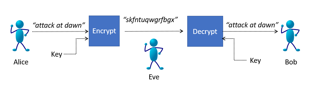
Alice (the sender) encrypts the message attack at dawn using a special key (similar to a password) to Bob (the receiver) without Eve being able to intercept the message and understand it. Bob decrypts the encrypted cleartext (the ciphertext) using the very same key. This implies that Alice and Bob had to get together first to agree on a key.
12.1. The Caesar cipher
The first cryptosystem we will study is really silly, and is easy to break. However, there are some good ideas in this system that we can use later to make a more secure cryptosystem. For simplicity, assume that we are communicating using lower case characters from the Latin alphabet (i.e., a-z). We can relax those conditions later. The idea of the Caesar cipher is that for each character in the cleartext we shift the character some distance down the alphabet. For example, if we used a shift of three, then an a in the cleartext would turn into a d. A b would become an e, etc., and a w becomes z. What about x, y, and z? These wrap around to a, b, and c. If we index each character in the alphabet by its position then shifting a character amounts to adding the position of the character to the shift mod 26.
Why 26? Well, 26 is the number of characters in our alphabet.
a b c d e f g h i j k l m n o p q r s t u v w x y z 0 1 2 3 4 5 6 7 8 9 10 11 12 13 14 15 16 17 18 19 20 21 22 23 24 25
For example, to encrypt attack by a shift of ten we take the position of a, which is 0 and add 10 mod 26 = 10. The tenth letter of the alphabet is k.
| Cleartext | i | (i + 10) % 26 |
Ciphertext |
|---|---|---|---|
|
0 |
|
|
|
19 |
|
|
|
19 |
|
|
|
0 |
|
|
|
2 |
|
|
|
10 |
|
|
We can choose the shift in advance by choosing a random number between 1 and 26. In this case the shift is also the key that both Alice and Bob must agree on.
| The Caesar cipher is sometimes called the rotation cipher or the shift cipher. |
The process of decrypting is exactly the same, except rather than add the shift, we subtract the shift.
For example, given the ciphertext "kddkmu" and a shift of ten we compute ("k" - 10) % 26 = 0, and 0 is the position in the alphabet of the letter a.
| Ciphertext | i | (i - 10) % 26 |
Cleartext |
|---|---|---|---|
|
0 |
|
|
|
19 |
|
|
|
19 |
|
|
|
0 |
|
|
|
2 |
|
|
|
10 |
|
|
One important aspect of this cipher is that Alice and Bob must get together and agree on a private key (the shift) beforehand.
To implement the Caesar cipher we need to be able to turn a character into its position in the alphabet. For example, the letter m into 12. We also need to be able to perform the inverse operation. Given the position in the alphabet what is the character at that position? For example, turning 12 back into m.
How can you turn a letter into its position in the alphabet?
Hint: Set up a variable alphabet initialized to the string "abcd...z".
What would the following print?
alphabet = "abcdefghijklmnopqrstuvwxyz"
print(alphabet.find('a'))
print(alphabet.find('z'))
print(alphabet.find('m'))Turning a letter into its position in the alphabet is a matter of calling the
find method on the string object alphabet.
0 (1)
25 (2)
12 (3)| 1 | The position of a |
| 2 | The position of z |
| 3 | The position of m |
How can you turn an integer from 0 to 25 into the corresponding letter?
Hint: What is the opposite of calling find? What would get printed by the following?
print(alphabet[0], alphabet[25], alphabet[12])
print(alphabet[alphabet.find('x')], alphabet.find(alphabet[23]))a z m (1)
x 23 (2)| 1 | The characters at positions 0, 25, and 12. |
| 2 | Indexing and find are inverses of each other in this case. |
Lets put this all together to implement a function encrypt that takes a cleartext message and a shift and produces a ciphertext as shown in the figure below.
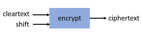
encryptimport string
def encrypt(cleartext,shift):
alphabet = string.printable (1)
ciphertext = '' (2)
for ch in cleartext: (3)
chpos = alphabet.find(ch) (4)
cipherpos = (chpos + shift) % len(alphabet) (5)
ciphertext += alphabet[cipherpos] (6)
return ciphertext| 1 | This is where we make it more general and handle any printable character. Not just lower case a to z. |
| 2 | ciphertext is initially empty. |
| 3 | For each character in cleartext. |
| 4 | Find the position of the character in the alphabet. |
| 5 | Compute the position of the ciphertext character. |
| 6 | Convert that position into a character. |
Calling
print(encrypt("Attack at dawn!", 13))prints NGGnpx7nG7qnJA. (including the period).
How do we write the function decrypt? Recall that decrypting is just subtracting the shift rather than adding. So the line
cipherpos = (chpos + shift) % len(alphabet)would change to
cipherpos = (chpos - shift) % len(alphabet)Or, rather than rewrite the entire function, we just notice that we could call encrypt with a negative shift.
print(encrypt("NGGnpx7nG7qnJA.", -13))and we get the original Attack at dawn! message.
So what is wrong with the Caesar cipher? Just about everything. But the main problem is that there are only as many different shift possibilities as there are characters in the alphabet, and it would be pretty easy to write a program to try them all.
12.2. Substitution Cipher
Lets try and fix the problem of the limited number of possible keys (shifts) and allow arbitrary mappings from a cleartext character to a ciphertext character. What if we were to use our scramble function on the alphabet to? For example …
alphabet = 'abcdefghijklmnopqrstuvwxyz'
key = scramble(alphabet)
print(key)Might print thubrwfzqpcjeovkmsgdxailny. In the substitution cipher an a would map to a t and a b would map to an h, and so on.
0 1 2 3 4 5 6 7 8 9 10 11 12 13 14 15 16 17 18 19 20 21 22 23 24 25 a b c d e f g h i j k l m n o p q r s t u v w x y z t h u b r w f z q p c j e o v k m s g d x a i l n y
Then to convert from a cleartext character to a ciphertext character it is as straightforward as finding the position of the cleartext character in the alphabet and returning the corresponding ciphertext character at that position. For example, using the key above, the expression key[alphabet.find('h')] would evaluate to the character z. The inverse operation needed for decrypting is, given a ciphertext character, find the corresponding cleartext character.
This is easy too. The expression alphabet[key.find('z')] would evaluate to h.
The function encrypt now takes a cleartext message and a key (i.e., a scrambled alphabet) and returns
the ciphertext. The function decrypt takes a ciphertext message and the same key that was used to generate the ciphertext, and returns the cleartext.
Write the functions encrypt and decrypt for the substitution cipher. Assume you can call the scramble function to generate a key that can be shared between encrypt and decrypt.
Here is encrypt.
def encrypt(cleartext, key):
alphabet = string.printable
ciphertext = ''
for ch in cleartext:
ciphertext += key[alphabet.find(ch)]
return ciphertextAnd here is decrypt.
def decrypt(ciphertext, key):
alphabet = string.printable
cleartext = ''
for ch in ciphertext:
cleartext += alphabet[key.find(ch)]
return cleartextHere is a main program that can be used to test encrypt and decrypt.
import string
key = scramble(string.printable) (1)
secret = encrypt("Attack at dawn!", key) (2)
print(decrypt(secret, key)) (3)| 1 | Create the key by scrambling all of the printable characters in python. |
| 2 | Encrypt Attack at dawn!. |
| 3 | Verify that what decrypt returns is indeed Attack at dawn!. |
Of course, once again, Alice and Bob must share the secret key, which this time is a little more difficult than sharing an integer shift. How many possible keys are there? A lot! Lets assume our alphabet is just the 26 lower case characters. The first character of the key can be any one of the 26 characters. The second character of the key can be any one of the 25 remaining characters, and so on. The number of possible keys is then \(26 \cdot 25 \cdot 24 \cdots 3 \cdot 2 \cdot 1 \). In mathematics this is 26 factorial, denoted as \(26!\). This is a very large number.
Write a simple Python program to compute 26 factorial.
There are lots of ways to do this. Here is one that matches the order of the operations \(26 \cdot 25 \cdot 24 \cdots 3 \cdot 2 \cdot 1 \)
prod = 1
for i in range(26,0,-1):
prod = prod * i (1)
print(prod)| 1 | You could also write prod *= i |
Of course, since multiplication is commutative (i.e., \(a \times b = b \times a\)) we do not have to start at 26 and count down. We could start at 1 and count up to 26.
prod = 1
for i in range(1,27): (1)
prod = prod * i
print(prod)| 1 | What would happen if our loop header was for i in range(27): |
Needless to say 26 factorial is 403291461126605635584000000. This number is larger than 4e26.
Surely the massive number of possible keys must mean that the substitution cipher is impossible
to break? Sadly, no. The substitution cipher is easy to break using a technique called frequency
analysis. To illustrate, let us once again assume we are dealing with the lower case Latin
alphabet and that Eve see’s the ciphertext hcchtrhclhyu. With a standard table of letter frequencies from https://en.wikipedia.org/wiki/Letter_frequency [Wikipedia] and a little patience a cryptanalyst could figure out that hcchtrhclhyu was attackatdawn. The weakness in the substitution cipher (and the Caesar cipher, as well as many other ciphers) is that letters repeat.
12.3. The One Time Pad - an Unbreakable Cipher
The One Time Pad combines the good idea of using addition modulo a random number with the randomness of a string of characters from the substitution cipher. The problem with the substitution cipher was that the key is only 26 characters long (or as long as the alphabet) and letters were reused thereby allowing a cryptanalyst to apply frequency analysis. What if we could generate a random string of characters that is as long as the message being encrypted? This random string of characters is the One Time Pad, which we will call the key. One again, for illustration, we will assume the lower case Latin alphabet.
To encrypt a message using a one time pad we line up the cleartext and the key (i.e., the one time pad) and add the positions of each character modulo 26. For example, encrypting apple using the one time pad lzksj results in the ciphertext lozdn.
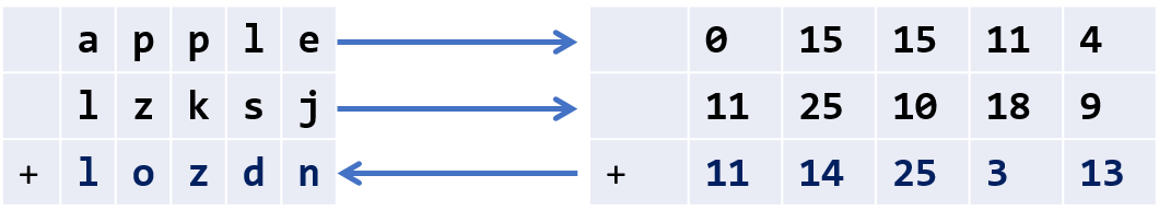
The process of decrypting using a one time pad is exactly the opposite. We line up the ciphertext with the key and then subtract modulo 26. For example, given the ciphertext lozdn we subtract the one time pad lzjsj to get apple back.
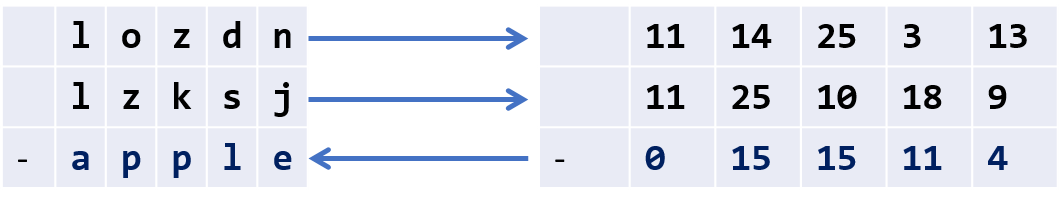
The one tricky aspect is to remember how to compute mod using negative numbers. For example, (14 - 25) % 26 is equal to -11 % 26 which is 15.
Implementing the encrypt and decrypt functions is straightforward.
def encrypt(cleartext, otp): (1)
alphabet = string.printable
ciphertext = ''
for i in range(len(cleartext)): (2)
ciphertext += alphabet[(alphabet.find(cleartext[i]) +
alphabet.find(otp[i])) % len(alphabet)] (3)
return ciphertext| 1 | The variable otp is the one time pad. Its length must be greater than or equal to the length of the cleartext. |
| 2 | We are using this version of the for-loop because we need to get the ith character from both the cleartext and the one time pad. |
| 3 | There is a lot packed in to this one line, but it simply looks up the position of a cleartext character and the corresponding one time pad character, adds them together mod the length of the alphabet to get the position of the ciphertext character, and extracts that character from the alphabet and concatenates it to the ciphertext. Note the use of the += operator. |
def decrypt(ciphertext, otp):
alphabet = string.printable
cleartext = ''
for i in range(len(ciphertext)):
cleartext += alphabet[(alphabet.find(ciphertext[i]) - (1)
alphabet.find(otp[i])) % len(alphabet)]
return cleartext| 1 | The only real difference between encrypt and decrypt is the - on this line. |
Why is the one time pad considered completely secure (unbreakable)? Recall that the pad must be as long as the cleartext being encrypted and that each character in the one time pad is truely random. Lets say we are presented with the ciphertext lozdn. In order to decrypt the first character l we would have to correctly guess the first character in the pad. We have a \(1/26 = .038\) chance of guessing correctly. To decrypt the first two characters we would have to correctly guess the first two characters of the pad, or \(1/26 \cdot 1/26 = .0015\) chance. To correctly guess the entire key of length five is \(1/26^5 = .000000084\). The message will be much longer than five characters so the
the probability of guessing all of the characters correctly quickly approaches zero.
If the One Time Pad is truly unbreakable then why aren’t all of our communications completely secure? Well, as you might expect the One Time Pad has a downside.
-
as the name suggests, the pad can only be used once. If you ever reuse a pad on a different cleartext, then the message is no longer secure because an attacker can now use frequency analysis to break the pad.
-
Since a one time pad must be as long as the cleartext message the pads could be really long. And since Alice and Bob both need to share a copy of the pad in advance then this could be cumbersome.
How does one go about generating a one time pad? This is relatively easy. Keep randomly picking characters from the alphabet and appending them to the pad.
Write a function GenOneTimePad that takes an integer n and returns a random string of characters of length n.
def GenOneTimePad(n):
pad = ''
alphabet = string.printable
for i in range(n):
pad += alphabet[random.randrange(len(string.printable))] (1)
return pad| 1 | There is actually a fatal flaw in our use of the standard random number generators in the random module. |
Random number generators found in programming languages are really pseudorandom. That is, the numbers generated are not really random but only appear to be random. They are fine for use in simulations such as Brownian motion or computer games, but their predictability make them unsuitable for cryptography or even games used in casinos. We say that they are not cryptographically secure. The acronyms we use for a pseudo random number generator is PRNG and the tongue twister cryptographically secure pseudo random number generator is CSPRNG.
Fortunately the Python module secrets provides a CSPRNG. A CSPRNG works by using a pool of genuine randomness called entropy. Entropy is built up over time, for example, times between keyboard presses, mouse movements, or network activity. It is also possible for a computer to run out of entropy! On some systems trying to generate a random number from a CSPRNG could actually block and have to wait until sufficient entropy is built up.
13. Tuples and Lists
Recall that a tuple is a value that contains a collection of values. For example we used a tuple for coordinates, such as (32,712) or (0,0). We used a tuple with three integers to specify colors, red is (255,0,0), and yellow is (255,255,0).
A tuple need not contain integers. Any time we want to think of several values as a single value we can use a tuple. For example, we can use a tuple to hold a name such as ("Harry", "Potter") which might be more helpful than storing the name as a single string "Harry Potter".
Tuples are also indexed like strings. Just like you can access the ith character in a string s as s[i], or the first character as s[0], we can index tuples as well.
name = ("Harry", "Potter")
print(name[1], name[0])prints Potter Harry. Tuples have a length:
print(len(name))prints 2.
We can also use tuples to hold a sequence of values. For example, a collection of grades.
grades = (98, 78, 72, 100, 85, 76)Because tuples are a sequence type we can iterate over them just like we can a string. To compute the average grade in grades …
1
2
3
4
5
6
total = 0
for g in grades:
total += g
avg = total / len(grades)
print("The average is", round(avg,2))
Like strings, tuples are immutable. Once a tuple is defined it cannot be changed. For example, using our grades tuple if we wanted to modify the first grade to be a 100 we might want to try …
grades[0] = 100causes a run-time error.
TypeError: 'tuple' object does not support item assignment
13.1. Lists
A list in Python is a lot like a tuple, except that it is mutable.
| A mutable value can be modified. |
When defining a list we use square brackets instead of parentheses to define lists.
grades = [98, 78, 72, 100, 85, 76]Because lists are mutable we can modify individual elements of the list.
grades[0] = 100 (1)| 1 | Replaces the 98 with 100. |
13.1.1. List methods
The list [] is the empty list whose length is zero.
grades = []
print(len(grades)) (1)| 1 | Prints 0. |
We can insert a value at the end of the list using the append method.
grades.append(78)
grades.append(83) (1)| 1 | The list is now [78,83]. |
This seems a little verbose since we could have just defined the list as
grades = [78,83]But we might not know the exact values in the list. What if they are coming from a file of grades? Or from the internet? For example, lets compute the median of a file of numbers? The median is the middle number, where half of the numbers are above and below the median. If there is an even number of numbers then the median is the average of the middle two numbers. One way to compute the median is to sort the numbers and pick the middle element. We can’t just read a number from the file, add it to an average, forgetting the previous number, like we did when we computed the average of a file of numbers in Example: Files of numbers.
To sort a list we can call the sort method on the list. The line
grades.sort()sorts the list of grades. The sort method returns None and has the side effect of modifying the list.
1
2
3
4
5
6
7
8
9
10
11
12
13
14
15
16
f = open('grades.txt')
grades = []
for grade in f: (1)
grades.append(float(grade))
grades.sort()
if len(grades) % 2 == 1: (2)
median = grades[len(grades)//2]
else: (3)
mid1 = grades[len(grades)//2 - 1] (4)
mid2 = grades[len(grades)//2]
median = (mid1 + mid2) / 2
print('Median:', round(median, 1))
| 1 | Append each grade in the file to the list. |
| 2 | For an odd length list, the median is in the middle. |
| 3 | Otherwise we need to compute the mean of the middle two elements. |
| 4 | Convince yourself that the grades at index len(grades)//2 - 1 and index len(grades)//2 are the middle two elements. |
13.2. The Birthday Paradox
The Birthday Paradox (also called the Birthday Problem) is a counterintuitive result in probability that asks how many people need to be in a room for there to be a 50% chance that two people share a birthday. As is often the case, many of our examples seem silly, but have real applications. In the area of computer security there is a particular type of attack called a birthday attack. The popular radio show This American Life did an episode titled Fraud Complex where the results from the birthday paradox were used to debunk claims of voter fraud.[36]
The mathematics for solving the birthday problem, while not all that complicated, is beyond the scope of this text. However, writing a program to simulate the birthday problem is fairly straightforward.
There are 366 possible birthdays (including the leap year day February 29). We can think of the calendar as a list of 366 integers. Call this list birthdays. The number of people in the room that share January 1 as a birthday is in birthdays[0] and the number that share December 31 is in birthdays[365]. Initially birthdays is initialized to all zeros.
1
2
3
4
birthdays = []
for i in range(366): (1)
birthdays.append(0)
| 1 | Append 366 zeros to the birthdays list. |
Python has an even simpler notation for initializing a list to all of the same value. The three lines of code above can be replaced with the one line …
birthdays = [0]*366How can we simulate someone’s birthday? Generate a random number between 0 and 365
and increment the corresponding birthday in the birthdays list.
1
2
bday = random.randrange(366)
birthdays[bday] += 1
We need to do this a number of times, once for each person in the room. How many times? This is precisely what we are trying to figure out. Lets start with 100.
1
2
3
for i in range(100): (1)
bday = random.randrange(366)
birthdays[bday] += 1
| 1 | Generate one hundred random birthdays. |
How do we know if two or more people share a birthday? One of the items in the birthdays list will be greater than 1. If nobody shared a birthday then all of the integers in birthdays are either 0 or 1. By the pigeonhole principle if there are 367 people in the room then we are guaranteed that at least two people share a birthday. In practice though, it is much less than that.
1
2
3
4
5
i = 0
for count in birthdays:
if count > 1:
print(count, "birthdays on day", i)
i = i + 1
Rewrite the above loop so that it uses the other form of a for-loop using the range function.
1
2
3
for i in range(len(birthdays)):
if birthdays[i] > 1:
print(birthdays[i], 'birthdays on day', i)
If we run this with 100 people in the room we see that lots of people share a birthday. (You will get different results because we are generating random birthdays).
2 birthdays on day 10 2 birthdays on day 23 2 birthdays on day 49 2 birthdays on day 69 3 birthdays on day 95 2 birthdays on day 144 2 birthdays on day 178 2 birthdays on day 290 3 birthdays on day 315 2 birthdays on day 316 2 birthdays on day 333
In fact with 100 people, you are almost guaranteed to have people share a birthday. With a little experimenting you can see that at about 23 people there is a 50% chance of two or more people sharing a birthday. It is called the Birthday Paradox because 23 seems like a surprisingly small number.
13.3. Particle Simulation: Take 2
Recall our particle simulation in Case study: Particles and Collision where we had two particles moving and colliding. For each particle we defined four variables x, y, dx, and dy. For two particles we need eight variables, and if we had six particles then we would need twenty-four variables. Also, our condition for checking collisions gets very long. We would have to check particle 1 against particles 2 through 6, particle 2 against particles 3 through 6
and so on. That would be \(5+4+3+2+1 = 15\) conditions. In general if we had \(n\) particles we need
\(n + (n-1) + (n-2) + \cdots + 3 + 2 + 1 = n(n-1)/2\)
conditions. So 100 particles would be \(4950\) conditions.
Rather than having separate variables for each x coordinate we can keep a list of x coordinates where x[0] is the x-coordinate for the first particle, x[1] for the second particle, and so on.
We will do the same thing for the y-coordinates.
x = [] # list of x-coordinates. x[i] is the x-coordinate for particle i
y = [] # list of y-coordinates. y[i] is the y-coordinate for particle iAssuming side is the height and width of the display and r is the radius of the particle (ball.get_width()//2) we can use two nested for-loops to distribute the particles evenly over the display.
1
2
3
4
for row in range(r, side, 6*r): (1)
for col in range(r, side, 6*r):
x.append(col)
y.append(row)
| 1 | Start at r so that the first particle is off of the edge a bit. Increment in steps of 6*r so that there is some space between the particles. |
We might want to verify that the code above works. We should check it by displaying the particles on the Pygame window.
Write a Python code fragment that would display the particles on the Pygame display.
We need to loop through all of the x and y coordinates and
blit each particle to the disaply.
for i in range(len(x)): (1)
win.blit(ball, (x[i], y[i]))
pygame.display.update()| 1 | We could have used the len(y) here as well. The two lists are the same length. |
And what we get should be something like the image …
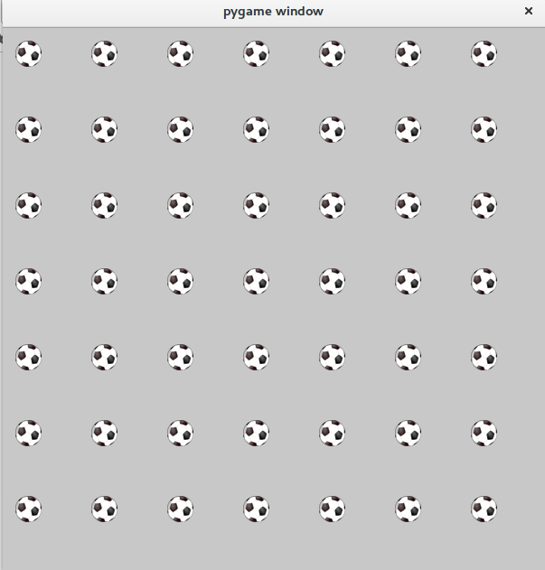
We also need to give each particle a velocity. And we want to give them different velocities, otherwise they would all move in the same direction at the same speed.
Since each particle will have its own velocity we will need a list of x-velocities and a list of y-velocities.
dx = [] # list of x-velocities. dx[i] is the x velocity for particle i
dy = [] # list of y-velocities. dy[i] is the y velocity for particle iWe saw that in our discussion of the frame rate (Understanding the Frame Rate) if the width of the window was 600 pixels and we set a particle’s x-velocity dx to 600 pixels per second, the particle would travel across the screen in one second. If we wanted the particle to travel across the screen in 2 seconds we would set dx to side/2 (or 300 pixels per second) assuming side is the width of the window. We want to give particles different velocities to make it look realistic. We can randomize the velocity of the particle between side/2 and side/4 seconds. For example, setting the x-velocity and y-velocity to side / (random.random() * 2 + 2)
Why does this work? Well random.random() * 2 gives a random value between 0 and 2 and adding 2 gives us a random value between 2 and 4.
But this means that all of the velocities are positive and all of the particles would be traveling to the right and down the display. We need some of the velocities to be negative, between -2 and -4. We have to be careful because we don’t want to generate values near 0 such as .001 because then side/.001 would be far too fast.

It is probably easiest to just toss a coin and randomly negate the value side / (random.random() * 2 + 2)
Our code for initializing the positions and velocities of each particle is …
1
2
3
4
5
6
7
8
9
10
11
12
13
14
15
16
17
18
19
20
21
22
23
24
25
import pygame, color, random
pygame.init()
side = 600
win = pygame.display.set_mode((side,side))
ball = pygame.image.load("../images/ball.png").convert_alpha()
r = ball.get_width()//2
for row in range(r, side, 6*r):
for col in range(r, side, 6*r):
x.append(col)
y.append(row)
# generate random velocities
tdx = side / (random.random() * 2 + 2) (1)
tdy = side / (random.random() * 2 + 2) (2)
if random.random() < .5: (3)
tdx = -tdx
if random.random() < .5: (4)
tdy = -tdy
dx.append(tdx)
dy.append(tdy)
| 1 | Generate a random x-velocity value between side/2 and side/4. |
| 2 | The same for the y-velocity. |
| 3 | Randomly negate the x-velocity. |
| 4 | And the same for the y-velocity. |
13.3.1. Moving the Particles
To move the particles we will use the same structure as we did when were animating just two particles. The main animation loop stays the same.
1
2
3
4
5
6
7
8
9
clock = pygame.time.Clock()
while True:
win.fill(color.lightgray)
dt = clock.tick(60) / 1000.0
# code to move and blit each particle goes here
pygame.display.update()
Back when we were animating two particles we had two separate calls to the
move function. If we had three particles we had three distinct calls to move. But here we are using lists and we want to move the ith particle.
(x[i],y[i],dx[i],dy[i]) = move(x[i],y[i],dx[i],dy[i])where i loops through all of thr particles.
for i in range(len(x)):
(x[i],y[i],dx[i],dy[i]) = move(x[i],y[i],dx[i],dy[i])
win.blit(ball, (x[i], y[i])) (1)| 1 | Don’t forget to blit the particle. |
Putting this all together we have the code to animate the particles.
1
2
3
4
5
6
7
8
9
while True:
win.fill(color.lightgray)
dt = clock.tick(60) / 1000.0
for i in range(len(x)):
(x[i],y[i],dx[i],dy[i]) = move(x[i],y[i],dx[i],dy[i])
win.blit(ball, (x[i], y[i]))
pygame.display.update()
13.3.2. Colliding the Particles
Assume we have \(n\) particles. We need to collide particle 0 with particles 1, 2, …, n-1 and particle 2 with 3, 4, …, n-1.
In general we collide particle i with particles i+1, i+2, …, n-1.
| Particle i | Collides with particles |
|---|---|
0 |
1, 2, 3, … , \(n-1\) |
1 |
2, 3, …, \(n-1\) |
… |
… |
\(n-3\) |
\(n-2\), \(n-1\) |
\(n-2\) |
\(n-1\) |
When we get to the last particle, \(n-1\), it has no other particles to collide with that we have not already checked.
1
2
3
for i in range(len(x) - 1): (1)
for j in range(i+1, len(x)): (2)
# collide particle i and j
| 1 | For every particle i except the last. |
| 2 | For every particle from i+1 to the last. |
Now we just add the conditional that if the distance between the centers of the two particles is less than two radii then they need to exchange velocities.
1
2
3
if distance(x[i] + r, y[i] + r, x[j] + r, y[j] + r) < 2 * r:
(dx[i], dx[j]) = (dx[j], dx[i])
(dy[i], dy[j]) = (dy[j], dy[i])
Putting it all together
1
2
3
4
5
for i in range(len(x) - 1):
for j in range(i+1, len(x)):
if distance(x[i] + r, y[i] + r, x[j] + r, y[j] + r) < 2 * r:
(dx[i], dx[j]) = (dx[j], dx[i])
(dy[i], dy[j]) = (dy[j], dy[i])
This goes in the main animation loop, which is now …
1
2
3
4
5
6
7
8
9
10
11
12
13
14
15
16
17
18
19
20
# main animation loop
clock = pygame.time.Clock()
while True:
win.fill(color.lightgray)
dt = clock.tick(60) / 1000.0
# move the particles
for i in range(len(x)):
(x[i],y[i],dx[i],dy[i]) = move(x[i],y[i],dx[i],dy[i])
win.blit(ball, (x[i], y[i]))
# collide the particles
for i in range(len(x) - 1):
for j in range(i+1, len(x)):
if distance(x[i] + r, y[i] + r, x[j] + r, y[j] + r) < 2 * r:
(dx[i], dx[j]) = (dx[j], dx[i])
(dy[i], dy[j]) = (dy[j], dy[i])
pygame.display.update()
13.5. Exercises
Suppose Alice creates a programming problem for HackerRank and a reviewer rates the question based on clarity, originality, and difficulty where each value is between 1 and 100. For example the tuple (90, 10, 50) means the problem is clear (90), not very original (10), and is of medium difficulty (50).
Suppose Bob also creates a problem for HackerRank with a rating of (75,50,60). We would like to compare Alice’s and Bob’s problems awarding a point for each criteria that is greater than the other’s. For example, in this case Alice’s score is 1 because her score on clarity is greater than Bob’s. Bob’s score is 2 because his problem is more original and harder. No point is allotted for values that are the same.
Complete the function compareTheTriplets below. It must return a tuple of two integers, the first being Alice’s score and second being Bob’s. The two paramaters are a, a tuple or list of three integers that represent Alice’s rating, and b, a tuple or list of three integers that represents Bob’s rating.
The input consists of two lines of three space separated integers. The first line is for Alice, and the second line is for Bob.
Sample Input 0
5 6 7 3 6 10
Sample Output 0
1 1
Sample Input 1
17 28 30 99 16 8
Sample Output 1
2 1
1
2
3
4
5
6
7
8
9
10
11
12
13
14
15
16
17
18
19
20
21
22
23
24
def compareTheTriplets(a,b):
# fill in function body
# M a i n P r o g r a m
# Don't worry about how the main program works
# Test Sample Input 0
if compareTheTriplets([5,6,7],[3,6,10]) == (1,1):
print("Sample Input 0 Passed")
else:
print("Sample Input 0 Failed")
# Test Sample Input 1
if compareTheTriplets((17,28,30),(99,16,8)) == (2,1):
print("Sample Input 1 Passed")
else:
print("Sample Input 1 Failed")
# Try your own inputs
a = [int(x) for x in input("Alice:").split()]
b = [int(x) for x in input("Bob:").split()]
print(' '.join([str(x) for x in compareTheTriplets(a,b)]))
Given a list of five integers find the minimum and maximum value that can be calculated by summing exactly four of the five values. For example, if the list was [7,9,3,1,5] the maximum would be \(7 + 9 + 3 + 5 = 24\) and the minimum would be \(7 + 3 + 1 + 5 = 16\).
Complete the miniMaxSum function below, where arr is a list of five integers. The function should return a tuple where the first item is the minimum sum and the second item is the maximum sum.
Sample Input 0
1 2 3 4 5
Sample Output 0
10 14
1
2
3
4
5
6
7
8
9
10
11
12
13
14
def miniMaxSum(arr):
# fill in function body
# M a i n P r o g r a m
if miniMaxSum([7,9,3,1,5]) == (16,24):
print("Sample Test 0 Passed")
else:
print("Sample Test 0 Failed")
# Try your own list of numbers
v = [int(x) for x in input("numbers: ").split()]
print(' '.join([str(x) for x in miniMaxSum(v)]))
Given a value k on one line and a list of integers on the second, complete the function twoSum below that returns true if two of the integers from nums add up to k.
Sample Input 0
25 4 9 33 2 16
Sample Output 0
True
because \(9+16=25\).
Sample Input 1
14 4 9 33 2 16
Sample Output 1
False
1
2
3
4
5
6
7
8
9
10
11
12
def twoSum(nums, k):
# fill in function body
# Try your own inputs
print(twoSum([4,9,33,2,16], 25)) # True
print(twoSum([4,9,33,2,16], 14)) # False
# Try your own k and list of integers
k = int(input("k: "))
nums = [int(x) for x in input("Numbers:").split()]
print(twoSum(nums,k))
This comes from the Daily Coding Problem email list.
Given a list of integers, return a new list such that each element at index \(i\) of the new list is the product of all the numbers in the original list except the one at \(i\).
For example, if our input was [1, 2, 3, 4, 5], the expected output would be [120, 60, 40, 30, 24]. If our input was [3, 2, 1], the expected output would be [2, 3, 6].
Follow-up: what if you can’t use division?
References and Reading
Students often ask me about books and resources. Here are some of my go-to references, when I’m looking for ideas, examples, or maybe just a new way to try and explain a difficult concept.
-
John MacCormick. Nine Algorithms that Changed the World. Princeton University Press. 2012.
-
Harrison Kinsley and Will McGugan. Beginning Python Games Development with Pygame. Second Edition. Apress. 2015.
-
Robert Sedgewick and Kevin Wayne. Computer Science, An Interdisciplinary Approach. Addison Wesley. 2017.
-
Mark Lutz. Learning Python. Fifth Edition. O’Reilly. 2013.
-
Bruce Schneier. Applied Cryptography. Second Edition. Wiley. 1996.
-
David Harel with Yishai Feldman. Algorithmics, The Spirit of Computing. Third Edition. Addison Wesley. 2004.
-
Iwo Bialynicki-Birula and Iwona Bialynicka-Birula. Modeling Reality, How Computers Mirror Life. Oxford University Press. 2004.
-
Sarah Flannery with David Flannery. In Code, A Young Woman’s Mathematical Journey. Algonquin Books of Chapel Hill. 2002.
-
Leonard Mlodinow. The Drunkard’s Walk, How Randomness Rules Our Lives. Pantheon. 2008.
-
David Harel. Computers Ltd. What They Really Can’t Do. Oxford University Press. 2000.
-
Ian Stewart. In Pursuit of the Unknown. Basic Books. 2012.
-
Elizabeth Allman and John Rhodes. Mathematical Models in Biology, An Introduction. Cambridge University Press. 2004.
-
Mitchell Resnick. Turles, Termites, and Traffic Jams, Explorations in Massivey Parallel Microworlds. The MIT Press. 1994.
-
Charles Petzold. CODE, The Hidden Language of Computer Hardware and Software. Microsoft Press. 2000.
-
Donella Meadows. Thinking In Systems, A Primer. Chelsea Green. 2008.
-
Nigel Gilbert. Agent Based Models. Sage Publishing. 2008.